Beating the correlation breakdown, for Pearson’s and beyond

JD Opdyke, Chief Analytics Officer, Sachs Capital Group Asset Management, LLC, shares his work and presentation on robust inference and flexible scenarios and stress testing for financial portfolios.

We live in a multivariate world, and effective modelling of financial portfolios, including their construction, allocation, forecasting, and risk analysis, simply is not possible without explicitly modelling the dependence structure of their assets. Correlation/concordance matrices like Pearson’s product moment correlation [1], Kendall’s Tau [2], and Spearman’s Rho [3] play a fundamental and central role here. As the scaled version of the variance-covariance matrix, Pearson’s rightly shapes our views and measurements of risk, diversification, and optimal construction and allocation in a very wide range of settings, from Markowitz efficient frontiers [4], to Black-Litterman scenarios [5] and fully flexible views [6], to BIS guidance on stress tests [7]. And while the limitations of Pearson’s are arguably often overstated [8] and/or misrepresented [9], when rank-based approaches are more appropriate, Kendall’s and Spearman’s are very widely used alternatives relied upon in all major financial settings [10].

Why, then, are these ubiquitous measures of correlation and dependence structure rarely treated in practice as rigorously estimated parameters like any others in these models? Why are values used for their cells in specified scenarios almost always ‘qualitative’ and informed by ‘judgment’ (if not arguably ad hoc) rather than probabilistically measured based on quantitatively determined finite sample distributions? When quantitative estimates are used, why are they rarely, if ever, associated with finite sample confidence intervals, both at the level of the entire matrix and that of the individual correlation cells, simultaneously and consistently? And why do these questions still apply to almost all stress tests ([11-14] are partial exceptions), even after major global financial crises and dramatically increased regulatory oversight worldwide? The latter is especially troubling given the widely documented ‘correlation breakdowns’ that occur during such times of extreme market stress [7,15-18], which is when risk analytics, and the (sometimes dire) consequences of the methods chosen for portfolio construction and allocation, matter the most [19-22].

Methodologically, I believe there are four major reasons for this less-than-ideal state of affairs, and only one approach that solves them all simultaneously.

Challenges

1. Efficient enforcement of positive definiteness

The first has to do with the requirement of (semi)positive definiteness, that is, the requirement that the correlation matrix represents data with (non-strictly) positive variances. This not only complicates the process of randomly sampling correlation matrices, but also requires very efficient algorithms when doing so. Simply ‘bootstrapping’ or perturbing the individual correlation values themselves will almost certainly generate non-positive definite matrices: in fact, if we were to randomly generate matrices that look like correlation matrices, with unit diagonals and off-diagonals ranging from –1 to 1, the chance of obtaining a positive definite matrix very quickly approaches zero as matrices become larger, even for fairly small matrices (e.g. for a 25x25 matrix, the probability is less than 2 in 10 quadrillion [23-28]). Although these specific numbers refer to Pearson’s, the same conclusion holds for Kendall’s and Spearman’s, and other positive definite measures of dependence.

2. Fully flexible perturbation/ scenarios

Closely related to 1. is the inability (until now) to vary individual (or selected groups of) correlation cells while holding constant the values of the remaining cells. This is an absolute requirement of fully flexible scenarios and accurate stress tests, since one financial crisis, and the corresponding changes in its correlation matrix, will look very different from the next (e.g. the dot-com technology bubble of 2000 vs the housing-crisis-induced recession of 2007-2008 vs the initial spread of Covid in 2020) [17,18]. But as described above, we cannot cavalierly ‘bootstrap’ or perturb the individual correlation cells, let alone the entire matrix, without violating the requirement of positive definiteness. To date, researchers have perturbed entire correlation matrices using methods that often or always preserve positive definiteness, and then simply ignored the unwanted effects on correlation cells that should be held constant (as dictated by the particular scenario or market crisis), referring to these ex post effects as ‘peripheral correlations’ [29,30]. Unfortunately, the distribution of the matrix where these ‘peripheral correlations’ are allowed to vary is quite different from that of the proper (constrained) matrix where they are not [23-27]. The underlying problem here is that most sampling approaches rely on spectral (eigenvalue) distributions which, while appropriate for analysing and understanding the p factors in a p-by-p portfolio, are simply at the wrong level aggregation for understanding the p(p-1)/2 pairwise associations amongst these p factors (e.g. for p=100, p(p-1)/2=4,950). The latter is far more granular than the former, and requires a method that directly accommodates this level of granularity (i.e. one that can explicitly link the distribution of a single correlation cell to that of the entire correlation matrix, and generate both simultaneously while preserving the flexibility of perturbing only selected cells).

3. Accuracy and robustness under general conditions

Lamentably, most research on sampling only positive definite correlation matrices has focused on narrowly defined, mathematically convenient cases (e.g. the Gaussian identity matrix) that have limited real-world application. Only rarely and recently have researchers focused on the general case [19, 20, 21, and arguably 22], requiring only the existence of the mean and the variance of the marginal distributions (for Pearson’s and Spearman’s) and the positive definiteness of the matrix (for all dependence measures). But of these few attempts, some rely on approximations that have been shown to be inaccurate as correlation values approach 1.0 [31,32], even though these correlation breakdowns are the very conditions under which stress and scenarios tests are most critically needed! Additionally, spectral distributions under general conditions are not as robust as those of the geometric angles of these matrices, either empirically, structurally, or distributionally, as described and used in the approach presented below.

4. One unifying framework across a broad class of widely used dependence structures

Defining the finite-sample densities of these measures of dependence unarguably is the necessary lynchpin to effectively modeling them – from inference and process monitoring to what-if scenarios to prediction – and to directly address and mitigate the effects of events like correlation breakdowns. However, only a handful of methods currently exist in the literature providing distributional results, and these are disparate [31, 33, 34], typically quite complicated [35,36], inflexible or unusable for testing and implementing granular, cell-level scenarios [31,32,37,38], and often limited to asymptotic results and/or unrealistic data assumptions [39,40,41]. What is needed is a single method for generating finite-sample distributions that can be applied not only across “the big three” correlations, but also to any measure of dependence that satisfies the fundamental and minimal requirement of positive definiteness (for example, see also the distance correlation of [42]). This would provide an advance in the literature with tremendous utility: practitioners and applied researchers would be able to isolate and compare, all else equal, using the same method, the behaviour of the various correlation/concordance measures under fully controlled, real-world data conditions. But to date, the extant literature has provided nothing close to this solution.

One solution: The unified framework of NAbC for dependence modelling

While many papers address one, and sometimes two of the four challenges above, none successfully address all four. Herein, I follow previous paths of research that utilise a geometric framework in this setting [43-46] to develop a method that overcomes all of them simultaneously, thus providing the finite sample distribution of any positive definite correlation/concordance matrix – including Pearson’s, Kendall’s, Spearman’s, and others – under general, real-world data conditions.

The non-parametric angles-based correlation (NAbC) method first obtains the Cholesky factorisation of the matrix. Next, the matrix analog of cosine similarity translates the Cholesky factor into a matrix of angles between the pairwise data vectors, and these angles retain all aspects of the data’s dependence structure [47,48]. Because the distributions of these angles are independent, this easily and efficiently generates not only marginal distributions corresponding to each cell’s (pairwise) correlation, but also a multivariate distribution corresponding to the entire matrix, simultaneously, and this multivariate distribution maintains excellent flexibility and robustness properties. Notably, the independence property allows for fully flexible perturbation of selected cells in the matrix, while holding the rest constant, via a simple, structured reordering of the matrix. No other approach provides this essential and necessary capability for granular, flexible scenarios and stress tests. And using angles distributions here rather than spectral distributions not only provides granular, cell-level flexibility, but also

1. efficiently and automatically enforces positive definiteness because the Cholesky factor places the angles on the unit hyper-(hemi)sphere; and
2. provides more accurate and more robust results when matrices approach singularity and/or extreme values.

This is due in part to the well-bounded range of the angles distributions (from zero to pi, rather than from zero to unbounded upper tails, which makes estimation less precise if not less accurate) as well as the non-parametric approach taken to estimating them. The latter not only contributes to robustness, but also ensures that the challenging characteristics of the underlying financial returns data (or that based on any copula function) – varying degrees of tail heaviness, serial correlation, non-stationarity, and/or asymmetry in the margins – pose no problems for NAbC, computationally or vis-à-vis empirical accuracy. Finally, in the general case with such real-world data, the method remains reasonably scalable (e.g. matrices 100x100, and larger), and under specific cases that can be fully defined analytically (e.g. the Gaussian identity matrix), sampling is more than 30% faster than the fastest competing methods [49] (see the implementation spreadsheet here [50]).

All results generated by NAbC are consistent with those well established in the Random Matrix Theory literature [51-53], even as NAbC remains more robust than methods based on spectral distributions. And the p-value it provides for the entire matrix can be used as a measure of ‘distance’ which, because it is defined probabilistically, has some advantages over traditional, norm-based metrics, as these arguably lack interpretation [54] and fail to attribute meaning to different relative distances of correlation values on a cell-by-cell basis.

In addition to all the above properties, NAbC remains far more straightforward and easily implemented than other approaches that provide more limited solutions to this problem. Its range of applications is extremely broad – as broad as the range of settings that rely on positive definite measures of dependence structure (which arguably defines the entire relevant usage space). The fact that the same, unifying method can define the distributions of this broad class of dependence measures is more than just icing on the cake: all-else-equal comparisons, consistently generated by the same method, will make apples-to-apples comparisons of previously incomparable results, and answer previously unanswered questions to very relevant, day-to-day challenges in portfolio analysis and management.

NAbC – Quantifiable answers to previously limited or unanswerable questions

While the above describes the major characteristics of the NAbC approach, and how it generates the finite sample distributions of positive definite dependence structures, below I list a dozen specific questions that now can be answered for having these distributions.

Given a specified or well-estimated correlation matrix [A], and its specified or well-estimated data generating mechanism:

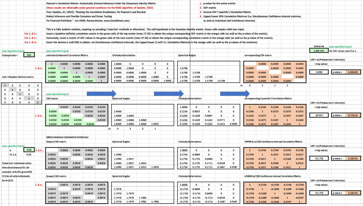
1. Confidence intervals:

What are the two correlation matrices that correspond to the lower and upper bounds of the 95% (or any) confidence interval for [A]? What are, simultaneously, the individual confidence intervals for each and every cell of [A]?

2. Quantile function:

What is the unique correlation matrix associated with [B], a matrix of cumulative distribution function values associated with the corresponding cells of [A]?

3. p-values:

Under the null hypothesis that an observed correlation matrix [C] was sampled from the data generating mechanism associated with [A], what is the p-value associated with [C]? And simultaneously, what are the individual p-values associated with each and every cell of [C]?

4.– 6: Scenario-constrained matrices:

For a specified scenario in which only some of the correlation cells in [A] change, and the rest are held constant, what are the answers to 1.– 3.?

7.– 12.: Direct comparisons across dependence measures:

What are the answers to 1.– 6. for, say, Pearson’s versus Kendall’s, or for comparisons between any positive definite measures of dependence structure? Having the finite sample distributions of these dependence measures, generated by the same method under the same real-world data conditions and scenarios, opens up a nearly limitless range of comparative inquiry for decision-making and statistical inference. For example, NAbC can be placed in statistical process control monitoring schemes wherein the distributions it provides can determine when one dependence measure has more power to detect regime changes than another, all else equal. And unlike other monitoring measures, this could be done with NAbC at (dimensional) scale and without requiring extensive Phase I burn-in simulations [55]. For inferential analyses generally, the relative precision and statistical power of, say, Szelsy’s (2007) distance correlation [42] versus Spearman’s would be essential and necessary information in the context of hypothesis testing. Robustness under extreme scenarios can be tested and compared for a given family of copulas, and the specific sources of more/less robustness of a given dependence measure identified under these controlled conditions: which characteristics of the copula function(s) and/or marginal distributions of the underlying returns data drive the answers to these comparative questions? Carefully crafted ‘what if’ scenarios are invaluable here and enable inquiry that can now provide answers rigorously and empirically and directly using NAbC. The list of critically important, applied research that NAbC facilitates, if not makes possible, is expansive and feasible with an ease of use and interpretability, broad range of application, scalability, and robustness not found in other more limited methods with narrow ranges of application.

With NAbC, we now have a powerful method enabling us to treat an extremely broad class of widely used dependence measures just like the other major parameters in financial portfolio models. We can use NAbC in frameworks that identify, measure and monitor, and even anticipate critically important events, such as correlation breakdowns, and mitigate and manage their effects. It should prove to be a very useful means by which we can better understand, predict, and manage portfolios in our multivariate world.

References

1. [1] Pearson, K., (1895), “VII. Note on regression and inheritance in the case of two parents,” Proceedings of the Royal Society of London, 58: 240–242.
2. [2] Kendall, M. (1938), "A New Measure of Rank Correlation," Biometrika, 30 (1–2), 81–89.
3. [3] Spearman, C., (1904), “’General Intelligence,’ Objectively Determined and Measured,” The American Journal of Psychology, 15(2), 201–292.
4. [4] Markowitz, H.M., (1952) "Portfolio Selection," The Journal of Finance, 7(1), 77–91.
5. [5] Black, F. and Litterman, R., (1991), “Asset Allocation Combining Investor Views with Market Equilibrium,” Journal of Fixed Income, 1(2), 7-18.
6. [6] Meucci, A., “Fully Flexible Views: Theory and Practice,” Risk, Vol. 21, No. 10, pp. 97-102, October 2008
7. [7] BIS, Basel Committee on Banking Supervision, Working Paper 19, (1/31/11), “Messages from the academic literature on risk measurement for the trading book.”
8. [8] Smirnov, P., et al, (2022) “Evaluation of Statistical Approaches for Association Testing in Noisy Drug Screening Data,” Bioinformatics, 23:188.
9. [9] van den Heuvel, E., and Zhan, Z., (2022), “Myths About Linear and Monotonic Associations: Pearson’s r, Spearman’s ρ, and Kendall’s τ,” The American Statistician, 76:1, 44-52,
10. Handbook of Heavy Tailed Distributions in Finance: Handbooks in Finance, Book 1 (Volume 1), 1st Edition, by S.T Rachev (Editor), North Holland; (March 19, 2003).
11. Chmielowski, P., (2014), “General covariance, the spectrum of Riemannium and a stress test calculation formula,” Journal of Risk, 16(6), 1–17.
12. Parlatore, C., and Philippon, T., (2022), “Designing Stress Scenarios,” NBER Working Paper 29901.
13. Packham, N., and Woebbeking, F., (2023) ,“Correlation Scenarios and Correlation Stress Testing,” Journal of Economic Behavior and Organization, 205:55-67.
14. Ho, Kwok-Wah, (2016), “Stress Testing Correlation Matrix: A Maximum Empirical Likelihood Approach,” Journal of Statistical Computation and Simulation, 86(14), 2707-2713.
15. Nawroth, A., Fabrizio, A., and Akesson, F. (2014), “Correlation Breakdown and the Influence of Correlations on VaR,” working paper, https://ssrn.com/abstract=2425515
16. Loretan, M., and English, W., (2000), “Evaluating ‘Correlation Breakdowns’ During Periods of Market Volatility,” Board of Governors of the Federal Reserve, International Finance Discussion Papers, Number 658.
17. Li, D., Cerezetti, F., and Cheruvelil, R., (2021), “Correlation Breakdowns, Spread Positions, and CCP Margin Models,” Securities and Exchange Commission, working paper, https://ssrn.com/abstract=3775828
18. Feng, C., and Zeng, X., (2022), “The Portfolio Diversification Effect of Catastrophe Bonds and the Impact of COVID-19,” working paper, https://ssrn.com/abstract=4215258
19. Salmon, Felix, (2008) “Recipe for Disaster: The Formula That Killed Wall Street,” WIRED, February 23, 2009.
20. BIS, Basel Committee on Banking Supervision, Working Paper 152, (March 2009), “Range of practices and issues in economic capital frameworks.”
21. BIS, Basel Committee on Banking Supervision, Working Paper 122, (June 2011), “Operational Risk – Supervisory Guidelines for the Advanced Measurement Approaches.”
22. Watts, S., (2016), “The Gaussian Copula and the Financial Crisis: A Recipe for Disaster or Cooking the Books?” working paper.
23. Opdyke, JD, (2020), “Full Probabilistic Control for Direct & Robust, Generalized & Targeted Stressing of the Correlation Matrix (Even When Eigenvalues are Empirically Challenging),” QuantMinds/RiskMinds Americas, Sept 22-23, Boston, MA.
24. Opdyke, JD, (2022), “Beating the Correlation Breakdown: Robust Inference and Flexible Scenarios and Stress Testing for Financial Portfolios,” QuantMindsEdge: Alpha and Quant Investing: New Research: Applying Machine Learning Techniques to Alpha Generation Models, June 6.
25. Opdyke, JD, (2022), “Beating the Correlation Breakdown: Robust Inference and Flexible Scenarios and Stress Testing for Financial Portfolios,” RiskMinds International / RiskFuse, December 6.
26. Opdyke, JD, (2023), “Beating the Correlation Breakdown: Robust Inference and Flexible Scenarios and Stress Testing for Financial Portfolios,” QuantStrats10, QuantStrategy & Innovation, NYC, March 14.
27. Opdyke, JD, (2023), “Beating the Correlation Breakdown: Robust Inference and Flexible Scenarios and Stress Testing for Financial Portfolios,” Columbia University, NYC–School of Professional Studies: Machine Learning for Risk Management, Invited Guest Lecture, March 20.
28. Pourahmadi, M., Wang, X., (2015), “Distribution of random correlation matrices: Hyperspherical parameterization of the Cholesky factor,” Statistics and Probability Letters, 106, (C), 5-12.
29. Ng, F., Li, W., and Yu, P., (2014), “A Black-Litterman Approach to Correlation Stress Testing,” Quantitative Finance, 14:9, 1643-1649.
30. Yu, P., Li, W., Ng, F., (2014), “Formulating Hypothetical Scenarios in Correlation Stress Testing via a Bayesian Framework,” The North American Journal of Economics and Finance, Vol 27, 17-33.
31. Hansen, P., and Archakov, I., (2021), “A New Parametrization of Correlation Matrices,” Econometrica, 89(4), 1699-1715.
32. Lan, S., Holbrook, A., Elias, G., Fortin, N., Ombao, H., and Shahbaba, B. (2020), “Flexible Bayesian Dynamic Modeling of Correlation and Covariance Matrices,” Bayesian Analysis, 15(4), 1199–1228.
33. Wang, C., Du, J., and Fan, X., (2020), “High-dimensional Correlation Matrix Estimation for General Continuous Data with Bagging Technique,” Machine Learning, 111:2905-2927.
34. Weichao, X., Yunhe, H., Hung, Y., and Zou, Y., (2013), “A Comparative Analysis of Spearman’s Rho and Kendall’s Tau in Normal and Contaminated Normal Models,” Signal Processing, 93:261-276.
35. Barber, R., and Kolar, M., (2018), “ROCKET: Robust Confidence Intervals via Kendall’s Tau for Transelliptical Graphical Models,” The Annals of Statistics, 46(6b), 3422-3450.
36. Niu, L., Xiumin, L., and Zhao, J., (2020), “Robust Estimator of the Correlation Matrix with Sparse Kronecker Structure for a High-Dimensional Matrix-Variate,” Journal of Multivariate Analysis, 177.
37. Ghosh, R., Mallick, B., and Pourahmadi, M., (2021) “Bayesian Estimation of Correlation Matrices of Longitudinal Data,” Bayesian Analysis, 16, Number 3, pp. 1039–1058.
38. Papenbrock, J., Schwendner, P., Jaeger, M., and Krugel, S., (2021), “Matrix Evolutions: Synthetic Correlations and Explainable Machine Learning for Constructing Robust Investment Portfolios,” Journal of Financial Data Science, 51-69.
39. Hamed, K.H., (2011), “The Distribution of Kendall’s Tau for Testing the Significance of Cross-Correlation in Persistent Data,” Hydrological Sciences Journal, 56(5).
40. Tsukada, S., (2021), “Asymptotic Distribution of Correlation Matrix Under Blocked Compound Symmetric Covariance Structure,” Random Matrices, 11(02).
41. Makalic, E., Schmidt, D., (2018), “An efficient algorithm for sampling from sin(x)^k for generating random correlation matrices,” arXiv: 1809.05212v2 [stat.CO].
42. Szekely, G., Rizzo, M., and Bakirov, N., (2007), “Measuring and Testing Dependence by Correlation of Distances,” The Annals of Statistics, 35(6), pp2769-2794.
43. Taraldsen, G. (2021), “The Confidence Density for Correlation,” The Indian Journal of Statistics, 2021.
44. Pinheiro, J. and Bates, D. (1996), “Unconstrained parametrizations for variance-covariance matrices,” Statistics and Computing, Vol. 6, 289–296.
45. Rebonato, R., and Jackel, P., (2000), “The Most General Methodology for Creating a Valid Correlation Matrix for Risk Management and Option Pricing Purposes,” Journal of Risk, 2(2)17-27.
46. Rapisarda, F., Brigo, D., & Mercurio, F., (2007), “Parameterizing Correlations: A Geometric Interpretation,” IMA Journal of Management Mathematics, 18(1), 55-73.
47. Fernandez-Duran, J.J., and Gregorio-Dominguez, M.M., “Testing the Regular Variation Model for Multivariate Extremes with Flexible Circular and Spherical Distributions,” arXiv:2309.04948v2
48. Zhang, Y., and Songshan, Y., (2023), “Kernel Angle Dependence Measures for Complex Objects,” arXiv:2206.01459v2
49. Rubsamen, Roman, (2023), “Random Correlation Matrices Generation,” https://github.com/lequant40/random-correlation-matrices-generation
50. Opdyke, JD, (2023), “The Correlation Matrix--Analytically Derived Inference Under the (Gaussian) Identity Matrix,” http://www.datamineit.com/DMI_publications.htm
51. Marchenko, A., Pastur, L., (1967). "Distribution of eigenvalues for some sets of random matrices,” Matematicheskii Sbornik, N.S. 72 (114:4): 507–536.
52. Lillo, F., and Mantengna, R., (2005), “Spectral Density of the Correlation Matrix of Factor Models: A Random Matrix Theory Approach,” Physical Review E, 72, 016219, 1-10.
53. Livan, G., Alfarano, S., and Scalas, E., (2011), “Fine Structure of Spectral Properties for Random Correlation Matrices: An Application to Financial Markets,” Physical Review E, 84, 016113, 1-13.
54. Bongiorno, C., and Lamrani, L., (2023), “Quantifying the Information Lost in Optimal Covariance Matrix Cleaning,” working paper, arXiv:2310.01963v1
55. Ebadi, M., Chenouri, S., Lin, D., and Steiner, S., (2022), “Statistical Monitoring of the Covariance Matrix in Multivariate Processes: A Literature Review,” Journal of Quality Technology, 54(3): 269-289.