Data challenges in applications of machine learning to quant finance problems

Currently there is a lot of excitement about applying machine learning to various problems in quantitative finance, as witnessed by a large number of talks on machine learning at the latest QuantMinds conference. However, these techniques stand or fall on the availability of large quantities of high quality data. In this blog, Dr. Svetlana Borovkova, Associate Professor of Quantitative Finance at Vrije Universiteit Amsterdam and Head of Quantitative Modelling at Probability & Partners, discusses some of the data challenges quants face when applying machine learning methods and illustrates these challenges on a few use cases.
Recent years saw an unprecedented explosion of interest in applying AI and machine learning (ML) to a variety of quant finance problems, ranging from derivatives pricing and risk management to market forecasting and algo trading. In fact, AI and ML are now seen as the greatest enablers of competitive advantage in the finance sector. However, according to the recent study by Refinitiv, data issues are perceived as the biggest barrier to the adoption and deployment of ML in finance.
Why is this the case and what are these data issues?
Recall that almost any machine learning algorithm needs a large and well-designed training (and test) set. This is especially true for function approximation algorithms such as neural networks, which typically have hundreds of unknown parameters. Creating such a training dataset is a hard job, which can be extremely cumbersome and time-consuming, and sometimes even impossible, and yet, this is the main part of applying ML.
A typical application of ML to a specific problem consists of several steps:
- Gathering and pre-processing large and versatile training and test sets.
- Making choices about a specific ML methodology. In order to pick the right ML algorithm from the multitude of possibilities (e.g., neural network, random forest, support vector machines), we need to determine whether the problem at hand is essentially a classification, ranking or functional approximation problem.
- Training the algorithm.
- Testing the algorithm and interpreting the outcomes.
Executing the last three steps is a lot of fun for a quant, as it involves learning new cool algorithms (such as LSTM networks, LambdaMART, AdaBoost and others), playing with sophisticated software (such as Python’s TensorFlow 2.0) and observing (hopefully great) results of your efforts.
However, in our experience, it is the first step that takes the most time and effort, and it can lead to the greatest frustrations. We see, both in academic research and in practical implementation, that a quant who is involved in ML, typically spends 50% (but often as much as 80%) of his or her time and effort on data cleaning and pre-processing and only 20 to 50% on actual training and testing of ML algorithms.
No data, poor data, alternative data
Data problems we face when applying ML methods to quant finance fall into three main categories. First of all, there might be not enough data to effectively train your ML algorithm. This is often the case in market forecasting, trading and quant investing problems, especially if daily or even lower trading/rebalancing frequency is considered. We have only one history of price and quote data, i.e., one realisation of price time series rather than a multitude of different scenarios needed to effectively train a ML algorithm. So a healthy dose of scepticism is needed when a study reports a successful ML application for daily stock market forecasting, which was trained on, say, 10 years of daily data (just a few thousand observations) and tested on one year of data (250 observations) – a lot more data than that is needed to train even a small neural network.
The second problem is poor data quality (e.g., missing values) and an unbalanced design of the sample, i.e., large discrepancy between the sizes of different categories. This situation is typical of credit risk applications, as we will illustrate below.
Finally, ML applications are excellently suited to incorporating the so-called alternative data in your models, such as textual or image information, news and social media content or client-specific characteristics coming from alternative data sources. Such alternative data can make huge contribution to forecasting or classification power of an ML algorithm, but it is often unstructured and comes from a wide variety of sources. So turning it into a well-structured training set typically requires an enormous synchronisation and pre-processing effort. In our next blog, about using news and social media sentiment for market forecasting and trading with ML, we will discuss exactly these issues.
Machine learning and quant finance – a perfect match?
There are, however, quant finance problems which are excellently suited to ML and where we can simply generate an unlimited amount of data to feed into ML algorithms. Such applications are derivatives pricing, their risk management and valuation adjustments. The reason for this is that in these applications we are fairly confident about the mechanics of the generating stochastic process for the underlying (such as interest rate, FX or a stock). So in such cases, we can generate a large number of scenarios for the underlying parameters, compute the corresponding derivatives prices (and the greeks) and then feed this generated training set into our favourite ML algorithm, to “learn” the relationship between the underlying parameters and derivative’s values.
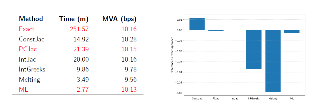
We have applied this idea to compute Margin Valuation Adjustments (MVA) for an interest rate swap book, in a use case for a major bank. Recall that computing margin valuation adjustment involves predicting future Initial Margin (IM) charged by a clearing house on (a portfolio of) derivatives, and these, in turn, are computed using the sensitivities of these derivatives to underlying factors (such as interest rates or volatilities). It is the precise calculation of these sensitivities that is usually cumbersome and time consuming. For example, numerical differentiation algorithms (the so-called “bump-and-revalue”) are inefficient and inaccurate. The modern technique of Algorithmic Adjoint Differentiation (AAD) does significantly better on both fronts, but can be still quite time-consuming (and complex). So we generated a large number of interest rate curves scenarios (100 000) in the two-curves setting – we used the two-factor Hull-White model – and then trained a deep learning algorithm (Feed-Forward Neural Network) to approximate the sensitivities of interest rate derivatives to the swap rates as a function of maturity, volatility and other parameters. The results were positive: the ML method had the same accuracy as different variants of AAD (e.g., constant Jacobian, piecewise Jacobian and so on), which is very hard to beat in terms of accuracy, but the MVA calculations with the trained ML algorithm were done in a fraction of time needed by AAD to obtain the same result, see table below for the actual comparison between the methods.
In other quant finance applications, we do not have the luxury of being able to generate our own training dataset. However, in many cases there is an abundance of data, such as in credit risk applications (e.g., predicting corporate or mortgage defaults). There, we usually have a large number of records for borrowers (mortgage or corporate loans), with their numerous characteristics, as well as the information whether the loan holder has defaulted/distressed or not. One such database is the so-called Orbis, which we used to train a ML algorithm to predict defaults of European small and medium companies (SMEs). The amount of data in Orbis is staggering: several millions of observations, covering the period 2006-2017. However, a closer look at the data reveals multiple problems: for a large proportion of companies, many records are missing or the information about the company (or the loan) is incomplete, and this is exacerbated for earlier years. So we designed a statistical interpolation algorithm to impute the missing values with the help of Principal Component Analysis, in combination with time series characteristics of the data. But of course, we could have used ML for this also!
Then the next problem, well-known in credit applications, presented itself. Only 5% of firms have defaulted and 95% did not (fortunately!), and this means that if we feed the dataset “as is” into a ML classifier (such as gradient boosting or random forest), the classifier will simply learn that most firms do not default and the predictive power of the algorithm will be zero. Fortunately, there are a multitude of methods to overcome this problem, ranging from heavy penalisation of not correctly classifying actual defaults to resampling schemes (such as SMOTE, Near Miss or RUS) that preferentially “draw” observations on the defaulted firms in the process of training of a ML algorithm. It turns out that penalisation does not work very well for default forecasting, but the Near Miss resampling scheme, in combination with gradient boosting, has delivered excellent results: defaults were correctly predicted in 90% of cases for the training set and in nearly 85% for the test set, beating by a significant margin traditional tools such as logistic regression. This is contrary to what is often observed in other credit-related ML applications, where the prevailing evidence is that it is hard to beat logit or probit regression. Our study shows that using a large quantity of carefully pre-processed data (in our case, statistically imputing the missing values), in combination with techniques to mitigate unbalanced design, does justice to ML methods which then outperform the traditional statistics.
So applying ML to quant finance turns a typical quant into a data analyst or data engineer, which is not necessarily a bad thing. It can be particularly exciting when new, alternative data sources are used in ML application, as we will discuss in our next blog about using news and social media sentiment in ML applications to algo trading.