High frequency markets’ volatility seasonality

Everything in our lives is based on our shared understanding of the measurement of time. Time tells you when to wake up and where you need to be, so it is no surprise that traditional methods of studying volatility was also dependent on time. But the periodicity of such measurements had a price, as detailed below by Vladimir Petrov, PhD research fellow of Marie Sklodowska-Curie initiative BigDataFinance at the University of Zurich, and Anton Golub, Founder and CEO, flov technologies. They propose a new approach to separate “the grains from the chaff”.
High-frequency trading (HFT) has never been more important for the world of finance than today. HFT highly automated algorithms submit, fill, and reject orders at ultra-high paces when a human does not even have enough time to blink. Two consecutive trades might literally happen as fast as a lightning: a thousandth fraction of a second is infinity in the HFT world. Professional trading companies build their data infrastructure with as high throughput as possible. Not just the fiber-optic, but straightly laid fiber-optic! All this complexity is needed to be the first in the queue of traders getting the market related information. Because if you are the first, you have the privilege to react to the information before others have managed to jump in front of you. High appetite to the financially related data leaves almost no room for the proper lightning-speed trading consequences assessment. This is why one needs to ex-ante collect as much information on the market’s properties pronounced at the ultra high-frequency scales as possible.
Such influential financial factor as volatility could not be left ignored by the curious scientific minds. Indeed, if you google “price volatility estimation” you will be provided with unprecedentedly long list of scientific literature on this topic. You could even understandably think that there should not be any problems anymore related to the volatility assessment. Of course, how could there be if researchers have already spent so many academic years to write the materials available online on how to estimate volatility. But such rich list of literature should also warn you that there might be some problems since the list has never stopped growing for so many years. Exactly, the problem is in the details.
Traditional methods of studying volatility are based on measures of periodicity which is defined in so-called physical time. In physical time, days, weeks, months, or years define the rhythm of events. Such periodicity-dependent measure performs pretty well for describing regularly occurring phenomena. For example, we all know that traders traditionally take a few days off within the Christmas period. It happens every year and it is pronounced in substantially decreased market activity. But there are plenty of such market events which can happen as instantly and severely hurt the system as well as become noticed only within a long period of time and result in the barely recognisable price changes. As a result, we risk to either miss the most important information if the fixed time interval between two measurements is too sparse or to get too much useless noisy records if the measurement periodicity is highly incessant. It is obvious that a better measure of time is needed to efficiently monitor and describe the erratic market’s dynamic.
A few decades ago Richard Olsen, a co-author of the published paper, together with his research colleagues proposed a new event-driven concept of time for finance. According to the concept, the evolution of the price curve itself is to dictate when a new observation should be made. The power of the approach, called directional-change intrinsic time, was proven by multiple highly cited research works. All those works leveraged the directional-change intrinsic time concept to reveal peculiar price curve properties formerly unknown. Market-making, high frequency trading, liquidity provisioning, and scaling laws discovering are among the brightest examples of the novel approach fruitfulness.
The utilitarian nature of intrinsic time can be employed to estimate the volatility in a new fashion. It is important to highlight that estimated by the novel method volatility is the actual volatility component of the stochastic process. That is the key difference of the method from the traditional techniques. The point is that high frequency market price curves are a dynamically evolving collection of various trends. The sequence of trends might even reveal some pattern for the external observer, but the patterns might be basely misleading. Noises, omnipresent in any time series, are to blame for that. Even the simulated price data, aimed at replicating the real market dynamic, has to be modelled as the composition of the trend component plus deterministic volatility part multiplied by some assumed stochastic noise. As a result, every time the volatility measured by the classical approach is the volatility mixed with the noise. The novel approach proposed in our paper is capable of separating the grains from the chaff: pure volatility part, exempt of the noise dust, is returned by the estimator.
Here and there, one can find various seasonality patterns characterising financial markets. The patterns are a natural phenomenon which emerges due to the traditional market architecture, which are big trading centres’ working days from Monday to Friday, and their employees’ lunch time in the middle of the day when they leave trading terminals to grab some food in the cafeteria nearby. Also, the geographical distribution of trading centres across the world unavoidably results in the particular seasonality patterns. Seasonality patterns are natural footprints of a particular market structure. Number of performed trades over time, accumulated volumes, size of the classical volatility are among these footprints to name a few. Numerous pages in multiple research papers thoroughly cover these and some other high-frequency market patterns. It is particularly important to highlight that the above-mentioned properties have not only the academic interest but are broadly considered by practitioners in a wide range of financial domains. Thinking about the novelty of the proposed instantaneous volatility evaluation method and about the omnipresence of the seasonality patterns, we decided to dive deeper and reconstruct the instantaneous volatility pattern on the one-week scale.
We have to admit that at the very beginning of the work there was no certainty on whether the directional-change seasonality can be found at all. Also, there was an important question which had to be answered before the research began: what markets should we select as the object of our study? It was clear that the “classical” markets, FX and stocks, have a well-explored set of seasonality patterns. But what about the novel markets and in particular highly provocative and yet insufficiently studied cryptocurrencies? Would anyone find any properties similar to those of classical FX and S&P 500 time series? Or would the set of discovered attributes be substantially increased or reduced due to the independent and unique blockchain architecture? Typically, if someone faces a similar question, he or she should address existing academic publication recently published in respected journals. So, we did. Only a few publications addressing cryptocurrencies seasonalities were available online at that time. The papers were mostly discussing traditional measures performed in physical time. We could not find any research work which would employ the directional-change intrinsic time concept to the promptly developing Bitcoin market.
Finally, we did not stint and decided to select all three markets for our analysis. Traditional approaches of estimating the realised volatility were considered too. That allowed us to directly compare the classical and the novel measures and highlight the benefits of each of them. Running ahead, quite a few surprising differences were found.
The fact that we found the direct connection of the number of directional changes to the instantaneous volatility is a major result for us. That is indeed the progress which potential we hope to further cultivate in a series of related scientific publications. But we are happy to say that there are also other important and curious findings.
It was shown in the research that the non-traditional cryptocurrencies market structure is pronounced in substantially different to FX and S&P 500 seasonality pattern. We found that the seasonality of the Bitcoin market is much less vivid. And yet, it still exists. That is particularly curious since Bitcoin is the best example of a new type of blockchain-powered assets freely traded all around the world without geographical or political restraints. There are no major Bitcoin trading centres where the big chunk of transactions would be processed or where the trading activity would be dictated by the working day agenda. The market is supposedly fully decentralised and has no middlemen (but we know it is not really the case, right?). Therefore, one could make an educated guess that the seasonality should be relatively flat. And it actually appears to be the case according to some of the recently published papers. But it is not anymore when looking at the market through the intrinsic time prism.
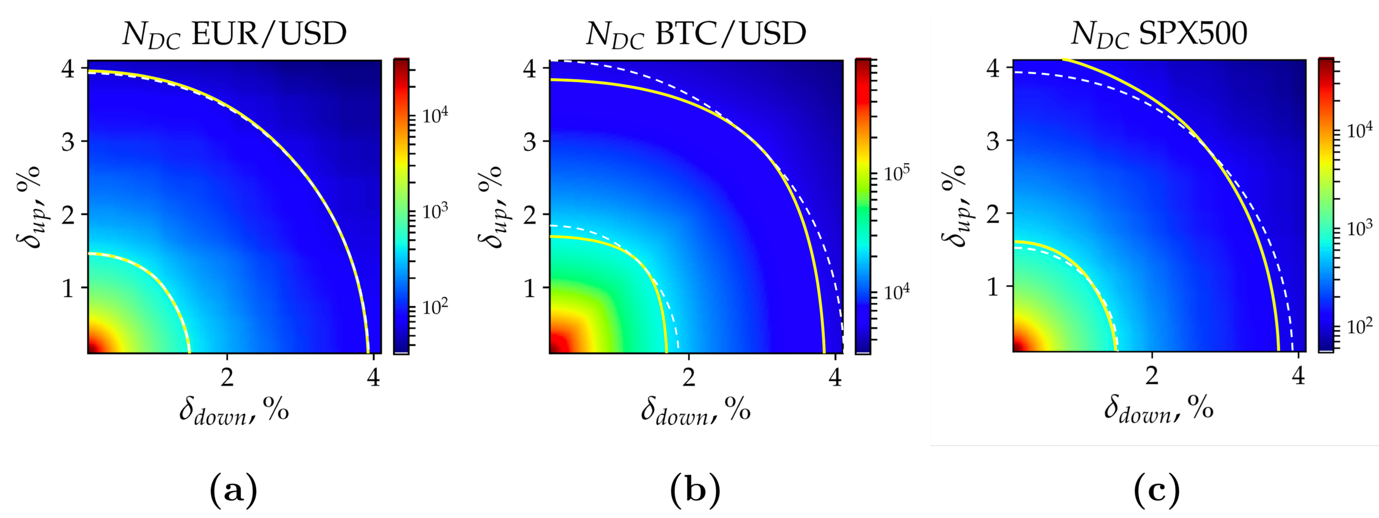 Figure 1: Heat map of the number of directional changes calculated in (a) EUR/USD, (b) BTC/USD, and (c) SPX500 time series. Each point on the grid represents the number of directional changes registered by a unique pair of thresholds {δup, δdown}. Heatmaps have different scales. Yellow solid lines, specific for each heatmap, label the examples of the areas along which the number of intrinsic events is constant. The dashed lines represent the theoretical areas of the equal number of intrinsic events observed in case of the trend-less time series. White dashed lines are parts of circles centred around the left bottom corner of each picture. The lines go through the intersection of the solid yellow lines and the diagonal of each picture
We also confirmed one of the reported observations that market participants from American and European regions have the biggest impact on the location of seasonality’s highs and lows. Just to explain: it is traditionally convenient to consider that there are three major trading zones in the world: American, European and Asian. It was documented long time ago that the market activity rises when one of those centres wakes up and falls at the corresponding end of the working day. Asia, despite being one of the most technologically advanced parts of the world, has a surprisingly low impact on the instantaneous volatility seasonality of Bitcoin versus American Dollar market. We tend to attribute the phenomenon to the fact that Asian governments, led by the Chinese one, forbid cryptocurrency trading, maybe because of the high level of novelties the technology brings to the financial system and the corresponding monitoring difficulties. Yet, we have no indisputable proof of the claim. Honestly, we are very curious to see how the seasonality dynamic will change over time while the blockchain technology gains broader acceptance and attract more professional market participants.
We have always been against the idea that a research work should be of interest only to one side of the scientific community: academics or practitioners. Therefore, we crafted the analysis in a way that it can be easily employed by both sectors.
The methods we developed could be used by other researchers as a building block for a set of new discoveries. For example, one of the most important academic works in finance is the option pricing model proposed by Nobel Prize winners Black and Scholes. The formula has one key component: volatility. There is no problem having the volatility in the formula assuming that real statistical price moves behaviour can be explained by the omnipresent in the physical world bell-shaped distribution. The bell-shape would simply dictate the probability of observing tiny price moves (a lot of them) as well as impressively big jumps (barely possible). But over decades of continuous work and after a few hundred of scientific publications the real price moves distributions is proven to be substantially deviated from the normal bell-shaped curve. The trading reality appears to be far from the ideal world. Research on intrinsic time in finance is an attempt to escape the stiffness of the traditional approaches. Intrinsic time research studies the price evolution from inside out. Thus, the distribution-like problems should not play any crucial role anymore.
The recently published research work is only one in the series projects we have been doing in our departments. The cornerstone of all studies is the directional-change intrinsic time applied to the high frequency financial data extracted from various markets. We have no doubt that you will like other publications we have planned for this year. Stay tuned!
Join Golub at QuantMinds International where he will be presenting on this.