Local volatility in interest rate model

Local Volatility (LV) is a very powerful tool to model market. This tool can be used to generate arbitrage-free scenarios calibrated to all available options. Here we demonstrate how to implement LV in order to calibrate interest model to all swaptions within a single model.
In 1994 Dupire [1] derived Local Volatility formula. This formula can be used to generate arbitrage free scenarios calibrated to all available options. Later, Gatheral [2] presented formula to express Local Volatility directly from implied volatility of market options. His formula made it easier to calculate LV. Also we have Local Volatility formula obtained for Normal Volatility Model [3].
Notice, that Local Volatility Model is the essential part of the process of generating calibrated scenarios in Local Stochastic Volatility (LSV) models. So, if we could implement LV then it can be applied in building of LSV to price exotic derivatives.
At first sight distribution of swap prices is not a normal or log-normal. It is a collection of bond price distributions. So, it is not correct to apply Local Volatility Model to calibrate interest rate model. However, as it was shown in [4], small volatility approximation works very well. It means that within this approximation swap distribution can be considered as a normal one. So, we can try to implement Local Volatility to calibrate interest rate model to all swaptions.
There are many interest rate models such as Hull-White model [5]; Heath, Jarrow, and A. Morton (HJM) [6], Libor Model [7]; SABR Model [8] etc. But currently, neither of them can be calibrated to all available swaption prices.
Here we demonstrate that LV can be implemented in HJM model to calibrate interest rate model and to obtain good calibrated swaption prices. The implementation is possible due to a good accuracy of this approximation. We are presenting detailed description of this implementation.
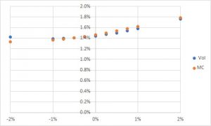
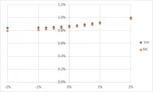
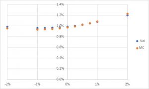
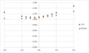
The results of 3/29/2022 SOFR swaption calibration are depicted in Figs.1-4. ”Vol” are input market volatilities and ”MC” are normal volatilities converted from swaption prices which are calculated by from Monte-Carlo in a single calibrated model.Figure 3: 2 Years Tenor 10 Figure 4: 10 Years Tenor 10
Figure 1: 2 Years Tenor
Figure 1: 2 Years Tenor
Figure 3: 2 Years Tenor 10
Figure 4: 10 Years Tenor 10
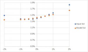
Notice, that short term calibration (see Figs.5,6) results can be improves by using shorter time steps or by using different from normal distributions with the same standard deviation as it was done in [9].
Figure 5: 0.5 Years Tenor 1
Figure 6: 0.5 Years Tenor 10
The other aspects of small volatility approximations were considered in [10].
In the presented implementation not all swaption prices are calibrated with satisfactory accuracy but it works well for most of them.
References
[1] Dupire, B. (1994). ”Pricing With a Smile.” Risk 7, pp. 18-20.
[2] Gatheral, J. (2006). ”The Volatility Surface: A Practitioner´ıs Guide.” New York, NY: John Wiley & Sons.
[3] Costeanu, V. & Pirjol D. ”Asymptotic expansion for the normal implied volatility in local volatility models” , arXiv:1105.3359v1, [ q-fin.CP, (2011);
[4] V.M. Belyaev : “Swaption Prices in HJM Model. Nonparametric Fit”, arXiv:1697.01619, [ q-fin.PR], (2016);
[5] Hull, J. and A. White (1990): ”Pricing interest-rate derivative securities”, The Review of Financial Studies, 3(4): 573−592.
[6] Heath, D., R. Jarrow, and A. Morton (1990): ”Bond Pricing and the Term Structure of Interest Rates: A Discrete Time Approximation”. Journal of Financial and Quantitative Analysis, 25: 419−440.
[7] Brigo, D. and F. Mercurio (2003). Analytical Pricing of the Smile in a Forward LIBOR Market Model. Quantitative Finance, 3(1), 15-27.
[8] Hagan Patrick S,. Kumar Deep, Kesniewski Andrew S., Woodward Diana E. (January 2002): ”Managing Smile Risk” Wilmott. Vol. 1. pp. 84–108.
[9] V.M. Belyaev : QuantMinds Americas Conference, Boston USA (2018).
[10] V.M. Belyaev : QuantMinds International Conference (2017-2021);
Viatcheslav Belyaev is Senior Quantitative Analyst at U.S. Bank. He will be presenting the above research at QuantMinds International. Don't miss his session, buy your ticket now.
