Looking over the horizon – with the help of bubble models

Historically, it has been quite impossible to predict the future, and in an exponentially evolving world and changeable market, the ability to know what is likely to happen before it happens has never been so valuable. Although financial bubbles have a bad name for being inefficient, Prof Dr Jerome L Kreuser, Senior Researcher, Department of Management, Technology and Economics, Zürich Switzerland and CEO and Founder of RisKontroller Global LLC, proposes that it can indeed produce meaningful information. So let’s see how Kreuser was able to predict the Bitcoin crash back in Dec 2017.
Modern Portfolio Theory (MPT) implies that historic returns are representative of future expected returns. Historical returns are random and expected returns are random as well. MPT has been described as driving a car forward while looking in a rearview mirror.
Can we do better before we have another major accident?
But is it possible to see over the horizon in financial markets and what does it mean?
Seemingly we couldn’t extract additional price information beyond the date of observation if markets are efficient. In addition, extracting reliable information from noisy markets (Black, 1986) characterised by a high noise-to-signal ratio are bound to fail. We look for those places where there can be market inefficiencies. One of those places with considerable prospects is bubbles, positive (resulting in crashes) or negative (resulting in rallies). There are several groups working on this thread including Kreuser and Sornette, 2018, Sornette and the Financial Crisis Observatory (2015 and many other references in Kreuser and Sornette, 2018), Davis and Lleo[1], 2015, Ziemba, Lleo, and Zhitlukhin, 2018, plus others.
There are several explanations for inefficiencies in financial bubbles. For example, Weinberger, 2014, suggests in an extension to Shannon’s Noisy Coding Theorem that a cause of market inefficiency in bubbles is that the underlying fundamentals are changing so fast that the price discovery mechanism simply cannot keep up. In the run-up to financial bubbles willful ignorance degrades the information processing capabilities of the market.
We suggest that in fact this process produces an increase in the amount of “pragmatic information” (meaningful information) in the market. The reason is that the noise-to-signal ratio is reduced in positive and negative bubbles because, assuming volatility is bounded, the expected return increases (sometimes exponentially). We know from Merton, 1980, and Ambarish and Seigel, 1996, that the time to estimate expected returns is a function of the ratio of volatility to expected return. We seek to exploit this in our bubble model and its applications in the following.
We have three main questions to answer.
- How to define the bubble model that is applicable to markets?
- How to estimate the parameters of that model?
- How to apply it to real markets?
We introduce the simple stochastic price process with a discrete Poisson process.
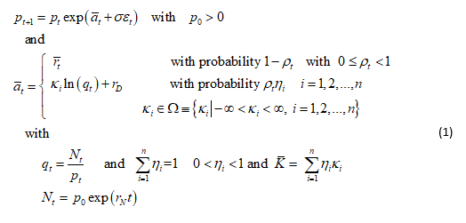
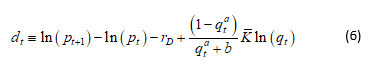
The crash factors, κ i , are assumed independent and constant over time and distributed according to the probability distribution Π≡{ηi = Pr[crash amplitude = κi]| i = 1, 2, ..., n}. Thus, conditional on no crash happening, which holds at each time step with probability 1-ρt, the price pt follows a geometric random walk with mean return ![]() on Δt and volatility σ. We assume that σ is constant, although it is not a necessary condition. At each time step, there is a probability pt for a crash/rally to happen with an amplitude that is proportional to the bubble size, or amplitude defined as
on Δt and volatility σ. We assume that σ is constant, although it is not a necessary condition. At each time step, there is a probability pt for a crash/rally to happen with an amplitude that is proportional to the bubble size, or amplitude defined as 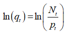 where Nt = p0exp(rNt) and rN is defined as the long-term average return[2].
We avoid trying to define what a bubble is. Rather we are concerned with jumps of any size. You may decide that a “bubble” is a “jump” of sufficient magnitude.
We assume now that the expected return ![]() is determined in accordance with the Rational Expectation condition
is determined in accordance with the Rational Expectation condition 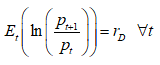 , which reads
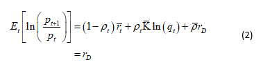
where ![]() is the expected crash factor. With the RE equation, the value
is the expected crash factor. With the RE equation, the value ![]() of the expected return of the risk asset is:
of the expected return of the risk asset is:

We form a Kelly (expected log of wealth) problem. Let λt be the fraction of wealth Wt allocated to the risky asset in time t and 1-λt the allocation to the risk-free asset with return rf. Then
where ![]() has been defined in (1). We wish to determine
has been defined in (1). We wish to determine 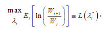 .
.
where Et is the expectation conditional on the information up to time t.
We estimate κi, ![]() , pt by separating the geometric random walk from jumps in the historical data. We do that using an extension of the method of Audrino and Hu (2016) on realised variation and bi-power variation. When we do that, we will separate out σ, meaning that a correct estimation of the model makes the “true” σ associated with the underlying geometric random walk component smaller than the apparent σ computed directly from the historical data without awareness that jumps are present.
, pt by separating the geometric random walk from jumps in the historical data. We do that using an extension of the method of Audrino and Hu (2016) on realised variation and bi-power variation. When we do that, we will separate out σ, meaning that a correct estimation of the model makes the “true” σ associated with the underlying geometric random walk component smaller than the apparent σ computed directly from the historical data without awareness that jumps are present.
This method produces an average probability for a crash/rally. After examining the following graph, we will discuss how we estimate a dynamic probability that is the crux of mitigating large bubbles and advantaging rallies.
We have the problem of estimating the parameters rD, rN, and the size of the time step [t, t+1]. This would seem problematic especially for rD, which can be very variable.
We approach the problem differently. We assume we now have an optimal Kelly process. We select a window of history to estimate the parameters. We select a suitable large matrix of varying value combinations and run the Kelly process on each. We select the set of parameter values that gives the optimal outperformance over the window of time as the “optimal” ones. We assume such a set exists and when we find it, we apply the same parameter settings over a subsequent window of time.
We apply this method in Figure 2 where we include graphs for:
- (Black) Optimal efficient portfolio: consisting of an optimal allocation between the asset and the risk-free rate,
- (Blue) Actual price: The actual price of the risky asset. All values and prices are measured in logs.
- (Violet) Normal price: Computed dynamically as explained above so it can change slope over time.
- (Green) BM Kelly portfolio: The classical Kelly allocation between the asset and the risk-free rate that quantifies risks solely based on return volatility.
- (Red) 60/40 portfolio: 60% in the asset and 40% in the risk-free rate.
We see in Fig. 2 that the Optimal Efficient Portfolio significantly outperforms the asset and most importantly it mitigates the DJ 1929 crash.
Fig. 2: Application of Kelly Process for DJ 1929 Data
Xiong and Ibbotson (2015) study accelerated stock price increases and note that they are strong contributors of a higher probability of reversal reconciling the 2–12 months momentum phenomenon and one-month reversal. This is further elaborated by Ardila-Alvarez, Forro, and Sornette (2016) who introduced the “acceleration” factor.
We introduce this factor by assuming a parametric form for the probability as a function of the mispricing for a positive bubble (q<1) and for a negative bubble (q>1) of the form:
For a positive or negative bubble, we have 0<qa≤1 and aln(q)≤0 ∀a as given above.
If we could measure ![]() , we could compute pt directly from equation (3). Along with the observable prices, we assume that the parameters rD, rN,
, we could compute pt directly from equation (3). Along with the observable prices, we assume that the parameters rD, rN, ![]() ,qt are known and from (3) and (5) define:
,qt are known and from (3) and (5) define:
We propose to calibrate the parameters a and b of the probability function using weighted least squares:
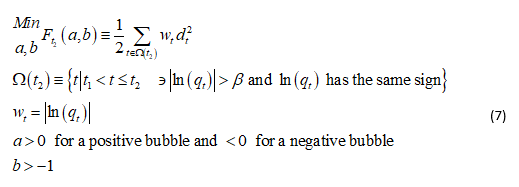
We define t1 as the beginning of a bubble when ln(qt) is close to zero and t2 the time when the probability is being estimated (i.e. “present” time). In practice, Ω consists of those time periods in a bubble where |ln(qt)| is sufficiently large as defined by the parameter β. The reason for β and the weights Wi is that the fit improves as |ln(qt)| gets large, i.e. when a bubble is well underway.
We are estimating ![]() through the RE equation. The reason this can work is that we have assumed that σ is constant (or at least bounded) whereas
through the RE equation. The reason this can work is that we have assumed that σ is constant (or at least bounded) whereas ![]() is accelerating. This also gives us the rational for weighting the observations by |ln(qt)| as, the larger it gets, the larger is
is accelerating. This also gives us the rational for weighting the observations by |ln(qt)| as, the larger it gets, the larger is ![]() .
.
Fig. 3 shows the values of the dynamic probabilities for the problem DJ 1929. Note that the crash probabilities keep jumping up throughout the runup to 1929 yet the Optimal Efficient Portfolio performs well with respect to the asset. In 1929 it mitigates the crash. The rally probabilities even predict the continued short-term rebound subsequently moving to zero as the price continues in downward run.
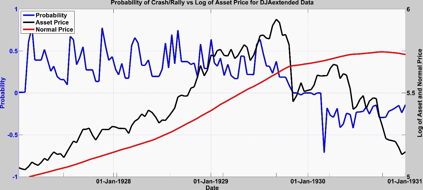
Fig. 3: Dynamic probabilities for the DJ 1929
Warren Buffet says he can’t beat the S&P 500 market (CNN Business: Markets Now: 25 February 2019 2:07 PM ET). So, should we try? We tried. We tested our bubble model over a 20-year period in Fig. 4 and ended up 2.7 times higher in total valuation or about an annualized improvement of about 5% additional return each year.
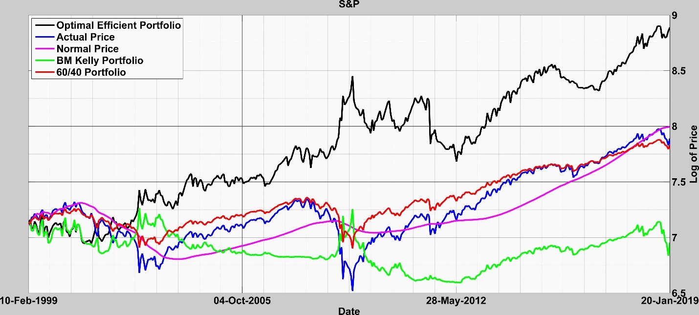
Fig, 4: S&P 500 over 20 years to today
The corresponding probabilities pt are given in the following Fig. 5.
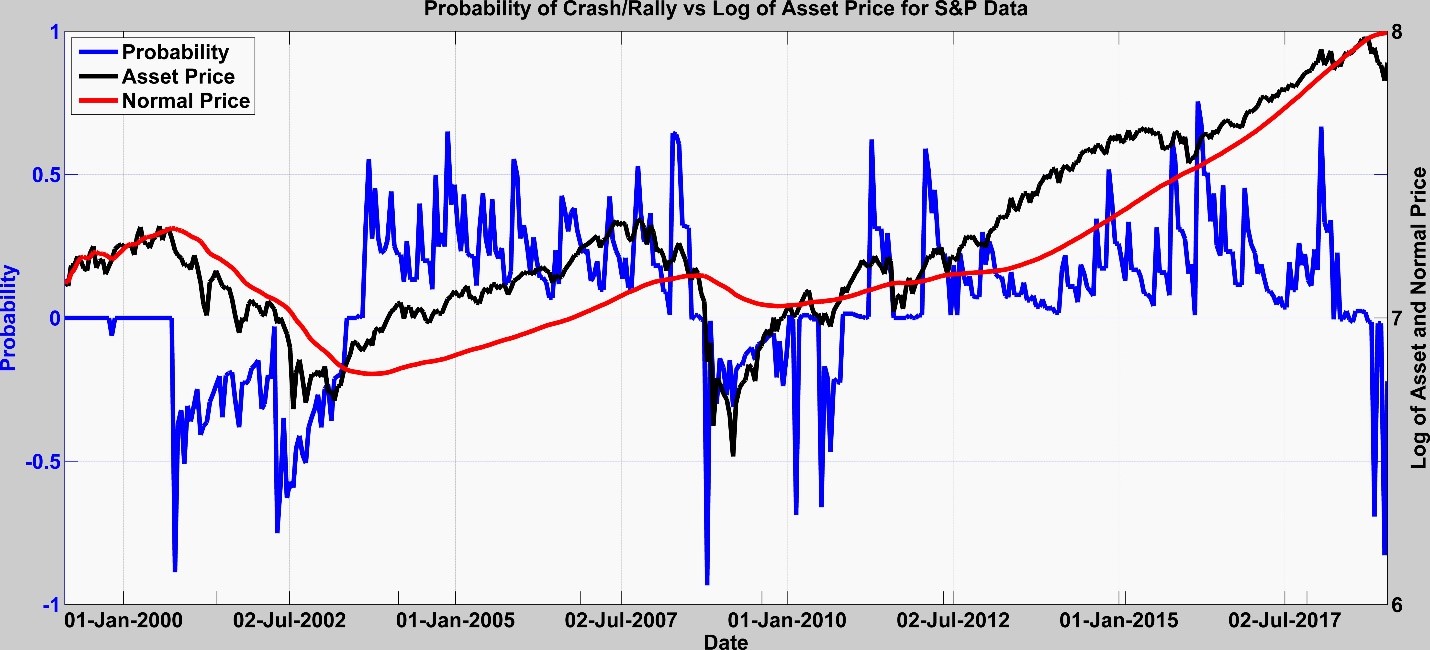
Fig. 5: Dynamic probabilities for the S&P 500 over 20 years
The probabilities were spiking two years prior to the 2007 crash and after the crash there was a rally probability signal indicating the recovery that occurred. We also see some probability spiking in 2017 followed by a substantial rally probability prior to the upturn, which isn’t indicated on this graph.
There has been a lot of talk in January about the possibility of an S&P crash. So, we ran our model and made a prognostication on 18 January 2019 (Details here). We detected no signal for a sustained crash. Rather we anticipated a slow movement toward the normal price while detecting probabilities for a rally (See Fig.6 & 7), which has occurred.
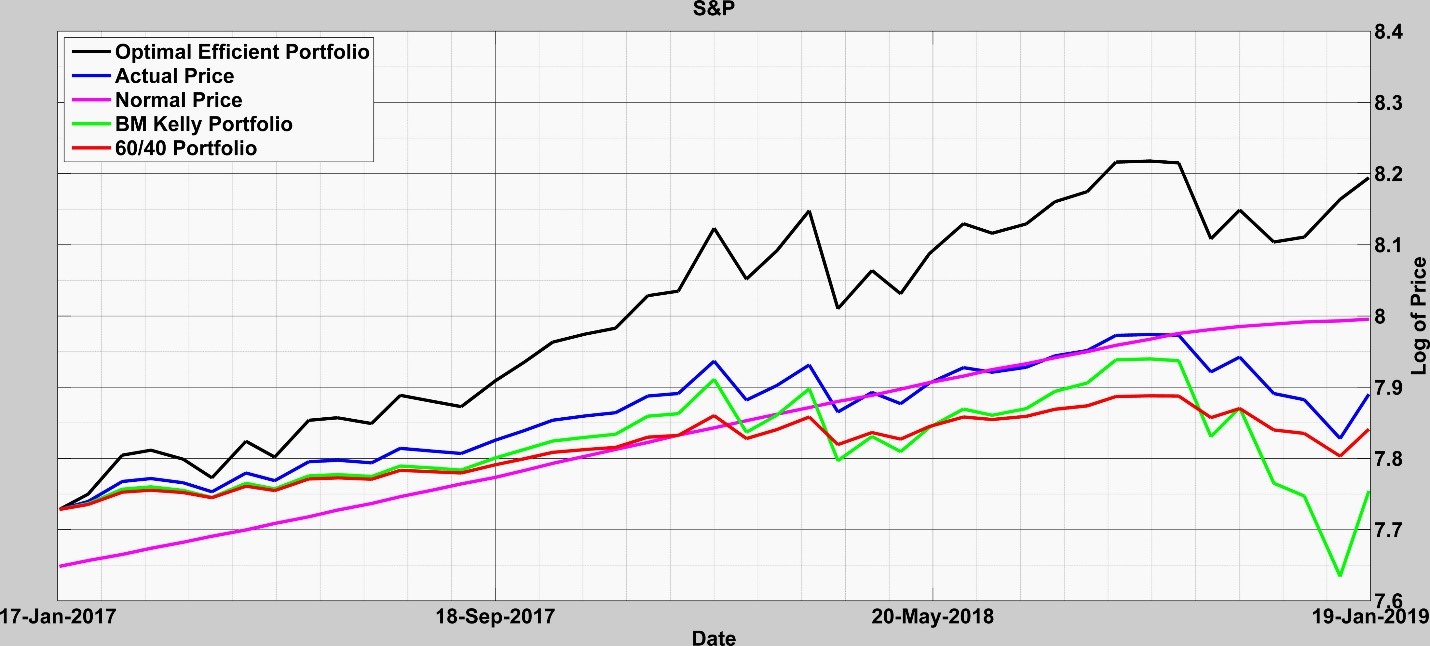
Fig. 6: model run over last year
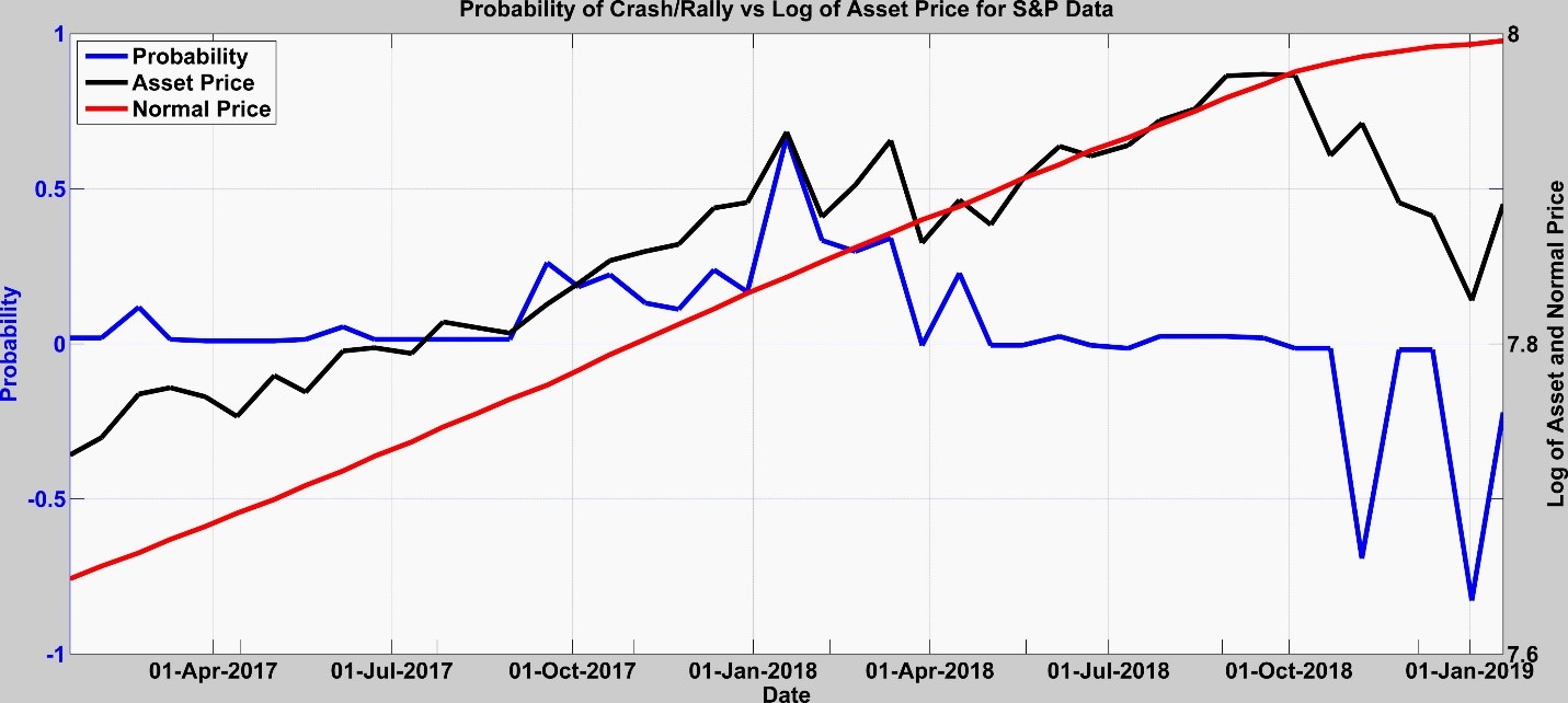
Fig. 7: Probabilities for S&P model run over last year
We give one last example. Using our bubble model on Bitcoin on 19-Dec-2017 we detected a sizeable bubble in Bitcoin and predicted it would crash and I recorded that possibility on LinkedIn on 21-Dec-2017. But there is much more. We predicted that the Bitcoin price would drop from 18,940 to 6,554 with a .78 probability. Our bubble model is based in part on the method of Kelly. So, it produces a portfolio composed of the asset and the “risk-free” asset. It showed in Table 1 that since August 2017 the model slowly divested itself of Bitcoin (See the parameter ) until by December 2017 it was almost fully divested of Bitcoin. The model yet showed an outperformance over Bitcoin of 265% over the period run. Details are in Kreuser and Sornette, 2018b. On 22 December 2018, I had sent two emails to the FT outlining these prognostications, which can be verified.
| Table 1: Kelly performance using our efficient Crash-bubble model on Bitcoin – Showing 1-Aug-2017 to 19-Dec-2017 but started 8-Jul-2013 | |||||
| Date | Crash Size (Crash Factor) | Crash Prob | Lambda λ | Efficient Portfolio Value | Price Bitcoin to USD |
| 01-Aug-17 | 1.35 | 0.29 | 0.60 | 27,705.45 | 2,731.00 |
| 15-Aug-17 | 1.67 | 0.24 | 0.52 | 36,419.50 | 4,155.67 |
| 29-Aug-17 | 4.41 | 0.17 | 0.42 | 38,370.18 | 4,578.82 |
| 12-Sep-17 | 2.28 | 0.28 | 0.35 | 36,968.03 | 4,172.56 |
| 26-Sep-17 | 2.28 | 0.14 | 0.71 | 36,106.87 | 3,888.03 |
| 10-Oct-17 | 2.28 | 0.62 | 0.17 | 41,767.13 | 4,749.29 |
| 24-Oct-17 | 1.22 | 0.73 | 0.10 | 42,950.55 | 5,523.40 |
| 07-Nov-17 | 1.22 | 0.64 | 0.15 | 44,239.07 | 7,130.28 |
| 21-Nov-17 | 1.22 | 0.61 | 0.18 | 45,159.44 | 8,095.23 |
| 05-Dec-17 | 0.68 | 0.71 | 0.05 | 48,795.59 | 11,677.00 |
| 19-Dec-17 | 0.68 | 0.78 | 0.00 | 50,206.47 | 18,940.57 |
 The model is complex enough to capture what needs to be captured. “Everything should be made as simple as possible, but not simpler.” Albert Einstein. An idea elegantly captured in the cartoon at the right.
Much yet needs to be done, verified, and improved. We are continuously working on it vigorously.
Can we see over the horizon? The view may be a bit fuzzy, but it seems we can see enough to make it profitable to look.

References
Ambarish, Ramasastry, and Lester Seigel. 1996. “Time is the Essence.” Risk (concord, Nh) 9 (8): 41–42.
Ardila-Alvarez, Diego, Zalan Forro, and Didier Sornette. 2016. The Acceleration Effect and Gamma Factor in Asset Pricing, Swiss Finance Institute Research Paper No. 15-30. Available at SSRN: http://ssrn.com/abstract=2645882.
Audrino, Francesco, and Yujia Hu. 2016. “Volatility Forecasting: Downside Risk, Jumps and Leverage Effect.” Econometrics 4 (8): 1–24. doi:10.3390/econometrics4010008.
Black, F. 1986. “Noise”, The Journal of Finance”, Vol. XLI, No. 3, July.
Davis, Mark H. A., and Sebastien Lleo. 2015. Risk-Sensitive Investment Management. Singapore:World Scientific Publishing.
Sornette, D. and P. Cauwels. 2015. “Financial bubbles: mechanisms and diagnostics”, Review of Behavioral Economics 2 (3), 279-305. See https://www.ethz.ch/content/specialinterest/mtec/chair-of-entrepreneurial-risks/en/financial-crisis-observatory.html
Kreuser, J. and D. Sornette. 2018. “Super-Exponential RE Bubble model with efficient crashes”, The European Journal of Finance, Volume 25, 2019 – Issue 4. Also see http://riskontroller.com/ and https://papers.ssrn.com/sol3/papers.cfm?abstract_id=3064668 .
Kreuser, J. and D. Sornette. 2018b. “Bitcoin Bubble Trouble”, Wilmott Magazine, May, and at SSRN https://papers.ssrn.com/sol3/papers.cfm?abstract_id=3143750 .
Merton, Robert C. 1980. “On Estimating the Expected Return on the Market.” Journal of Financial Economics 8: 323–361.
Weinberger, E. D. 2014. “Pragmatic Information Rates, Generalizations of the Kelly Criterion, and Financial Market Efficiency”, https://arxiv.org/ftp/arxiv/papers/0903/0903.2243.pdf .
Xiong, James X., and Roger Ibbotson. 2015. “Momentum, Acceleration, and Reversal.” Journal of Investment Management 13 (1): 1st quarter.
Ziemba, William T.; Sebastien Lleo; and Mikhail Zhitlukhin. 2018. “Stock Market Crashes”, World Scientific Series in Finance, Vol. 13.
Footnotes
[1]What we do different from Davis and Lleo is that we combine our bubble model with a discrete time Kelly
process whereas their jumps are independent of a bubble model and their model is in continuous time.
[2] We call it the “normal price return”. Some may interpret this as a fundamental price return but that is not the specific intention here.