Modelling during quantitative easing
The reversal of Quantitatve Easing (QE) has sent shivers down the spine of the market. US 10 year benchmark bond yields are at four year highs, and still rising. This has been contagious; accounting for at least some of the dramatic sell off in equities this year.
Managers of systematic strategies do not need to worry about trying to second guess the market; that is what their models are for. But they may wish to try and make meta-predictions; forecasts of how their models might do in particular market conditions.
To perform this kind of analysis we need two ingredients. First of all we need one or more strategies whose returns we can backtest historically. Secondly we need a conditioning variable to objectively identify various market regimes. The trick then is to partition historic strategy returns according to the regime that was present. We then see whether backtested returns are unusually high or low in past regimes that were most like the present.
Your choice of strategy is entirely to personal taste. For this article I’m going to use a momentum and a carry strategy. This closely matches my own trading system, but is also a good proxy for many systematic hedge funds. Managed futures funds, which are also known as commodity trading advisors (CTAs), tend to have a big slug of momentum in their models. Many fixed income strategies have a high Beta to carry.
QE has never happened before in the US, and has never been reversed before.
To make the analysis easier I’ll also be focusing on four markets: the US Eurodollar, and three bond futures. There will of course be spillover effects to other instruments, countries and asset classes; but we would expect to see the strongest effects of reversing US QE in US bonds and interest rate derivatives.
Identifying the conditioning variable is more difficult. We can’t really use QE itself. QE has never happened before in the US, and has never been reversed before. Instead we need to choose a variable with a long history which will work as a QE substitute.
A naive description of the effect of QE reversing would be something like this “interest rates are low, but have started rising”. The level and change of interest rates is a good proxy for the end of QE.
Importantly we need to make a choice between regimes that were identifiable ex-ante or ex-post. Identifying ex-post that a particular strategy did well or badly in a particular regime is of little practical use if the regime can’t be identified in advance. A regime based on official recession indications would be an example of this; the NBER doesn’t call the start or end of recessions until a year or so afterwards. So we need to use two ex-ante indicators: the level of interest rates before a given period, and the change in interest rates up to the start of that period.
Which interest rate should we use? The average maturity of US debt moves around, but averages around 5 years. The constant maturity 5 year yield of government debt is probably a decent measure of how QE has affected.
It’s problematic to use an un-adjusted level of interest rates, since interest rates have been trending down. Instead I’ve normalised interest rates by dividing the current rate by the 15 year average interest rate; giving us a measure of where we are in the monetary policy cycle. I’ve also divided the one year change in rates by recent average rates; arguably a 0.5% rise is more significant now than it was in the 1980s.
It turns out that the results for the level of rates are inconclusive, so in this post I’ll focus on analysing the effects of normalised changes in 5 year yields.
In figure 1 you can see the cumulative performance of our CTA replicating portfolio containing the four US fixed income futures trading both momentum and carry trading rules.
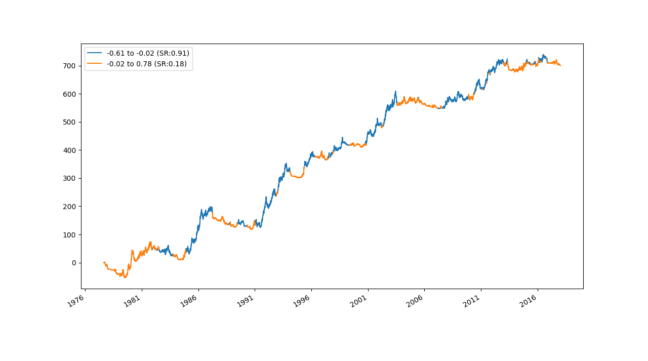
Figure 1
You can see that the performance when rates are rising (in orange) is inferior to a falling rate regime (in blue); the Sharpe Ratio falls from 0.91 to 0.18. The other figures in the legend show the range of normalised rate changes for each regime.
These results look compelling, but we need to check that they are statistically significant. Figure 2 shows the bootstrapped distribution of the Sharpe Ratio estimate for each regime.
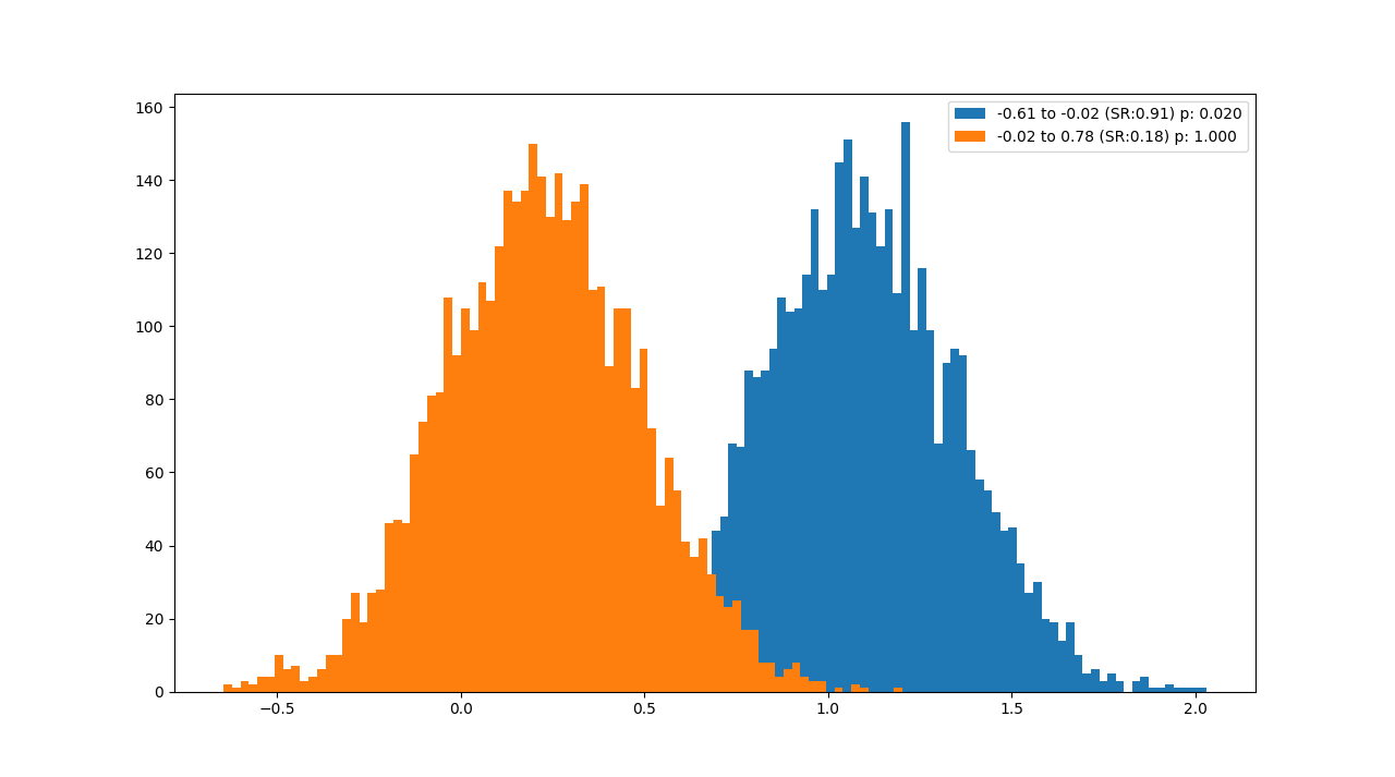
Figure 2
There certainly seems to be a distinct difference here, and the results of a formal t-test confirm that with a p-value of 0.02; implying there is a 98% chance that the Sharpe Ratio of fixed income strategies is higher when interest rates have recently been falling.
I’ve repeated this analysis for a number of different assets, and the results are shown in table 1 below:
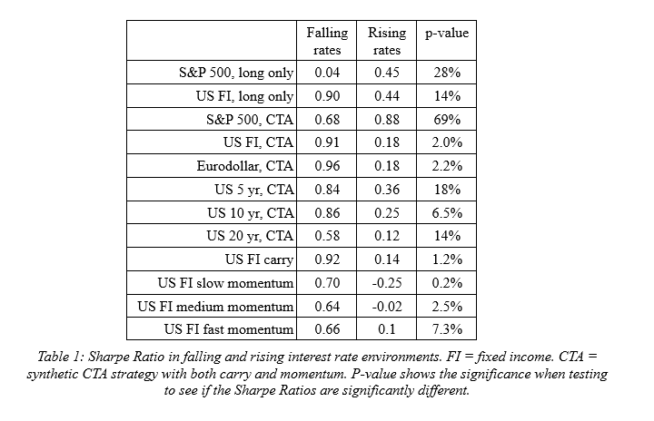
.
This gives us the following asset allocation recommendations, conditional on the current regime where interest rates have been rising:
- Long only portfolios: you may consider a relative reallocation to stocks away from bonds, but don't overdo it: even in the current environment historically bonds seem to have done just as well as stocks
- CTA allocations: a small deallocation from CTAs may be worthwhile but a well diversified CTA without too much fixed income exposure shouldn’t suffer unduly in the current regime
Systematic managers of CTAs may also wish to consider the following:
- Asset class allocations: You should downweight fixed income, and upweight other asset classes
- Strategy allocations: You should consider downweighting slower momentum strategies in favour of carry and faster momentum
Our attempt at meta-prediction has given us some indication of how rising yields might affect us, but none of the results are strong enough to justify completely removing anything from your portfolio. Instead small tweaks and gradual portfolio re-allocations should be the order of the day. Finally if you’re going to introduce a portfolio overlay based on interest rate regimes then it should be done systematically – be prepared to reverse any changes when rates begin to fall again.

Robert Carver is an expert on systematic trading and a guest lecturer at Queen Mary University of London; a former head of fixed income at multi billion dollar quantitative hedge fund AHL and former investment bank trader, and the author of two books: "Systematic Trading" and "Smart Portfolios". You can read an expanded version of this article here >>