Modelling volatility

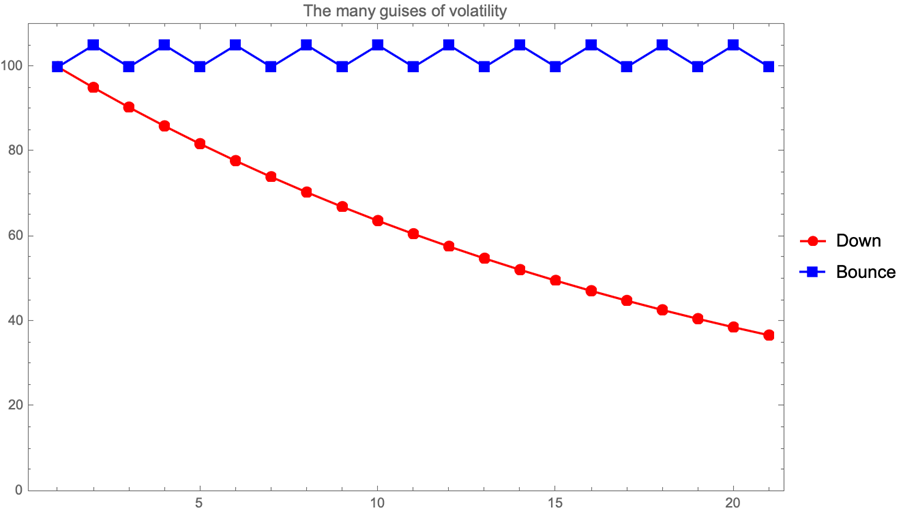
Sometimes we can become so focused in our research that we might be surprised by our failure to communicate with others using familiar terms (“I do not think it means …”). Take volatility as an example; while option traders might think about realized and implied volatility as statistics and formula inputs, a mathematician might think about a stochastic process with certain properties. How the volatility happens makes no difference for the payoff of a variance swap, but a regulator might have a different opinion which “volatility” should merit an intervention:
We might try to model processes with trends and covariances, but we might never be sure, given a particular time series, of which was which. Our temptation is to think of volatility as directionless and assign the rise or fall to a trend. While many books and articles delve into this problem with mathematical rigor and intricate detail, we want to discuss the challenge of estimating volatility from a conceptual point of view.
If we’re measuring volatility from price changes, we can think about either how many changes happened in a standard time period (e.g. 5 minutes or 8 trading hours, correcting for the size of the changes when appropriate) or how the time series of (e.g. daily) changes … changes (e.g. looking at the standard deviation of these changes).
In a previous presentation (“The Right Kind of Volatility”) I discussed the first case, where we infer the likely sets of (trend, volatility, discretization parameter) given price changes and the times between these changes. Looking at data, we can observe that the distribution of these times is coherent with a lognormal distribution of volatilities.
If we want to assign causes to these changes, we need to understand how markets work and build a model that goes from realistic behavior to testable consequences. From the point of view realistic behavior, one of the most promising choices is the use of Hawkes processes; they allow different kinds of agents to act according to their own standard behaviors and to react to the behaviors of others, reinforcing or dampening the intensity of the arrival of orders (a typical setup would have Limit and Market Orders and the Cancellations of Limit Orders).
From the statistical point of view, Rough Volatility models are able to explain the behavior of statistical measures of volatility, starting from their lognormal distribution as mentioned before, and fit implied volatility surfaces to price and hedge options. But their main advantage, in our opinion, comes from the link between the main stylized facts of market microstructure, encoded in Hawkes processes, and rough volatility as a consequence of these behaviors.
One way to think about why volatility must be rough (i.e. change a lot on different scales) is to think again about the times between price changes. If volatility did not change a lot even at this sub-minute scale, we would have price changes at regular intervals, meaning that the reactive part of the markets is much less frequent than the one driven by new information or flows. And if there was any doubt about the endogeneity of markets, the examples of sudden instability are too numerous to list here, from 2010’s Flash Crash to 1987’s Portfolio Insurance debacle; the time scales might be different, but markets, even in this computerized age, still resemble more Kal’s classic “Buy!Sell!” cartoon than a quiet and efficient order matching auction house.
One way to think about why volatility must be rough (i.e. change a lot on different scales) is to think again about the times between price changes. If volatility did not change a lot even at this sub-minute scale, we would have price changes at regular intervals, meaning that the reactive part of the markets is much less frequent than the one driven by new information or flows. And if there was any doubt about the endogeneity of markets, the examples of sudden instability are too numerous to list here, from 2010’s Flash Crash to 1987’s Portfolio Insurance debacle; the time scales might be different, but markets, even in this computerized age, still resemble more Kal’s classic “Buy!Sell!” cartoon than a quiet and efficient order matching auction house.
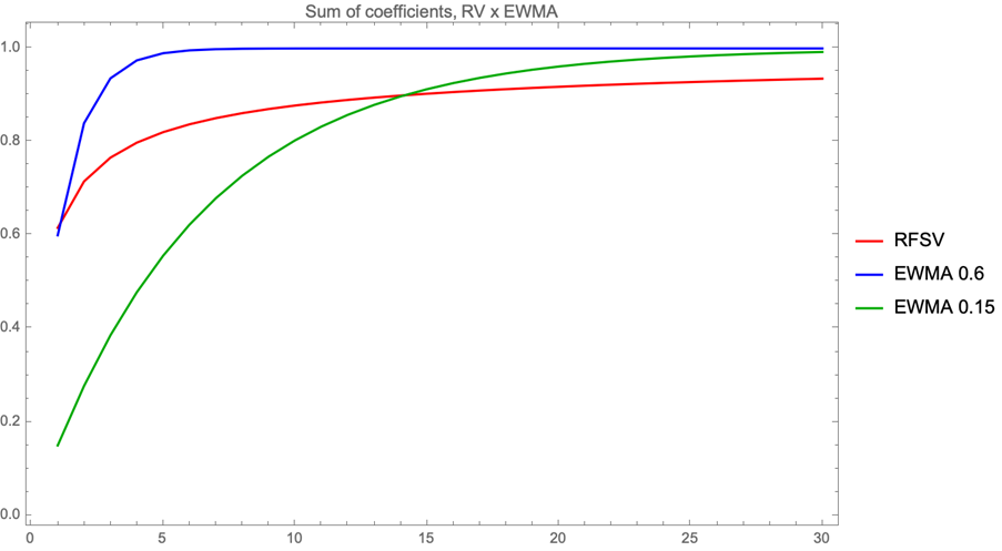
And the more interesting conclusion is that, in order to decay that slowly, the weights after a relatively low number of lags cannot be too different. In fact, the ratio of successive coefficients approaches 1 quite quickly:
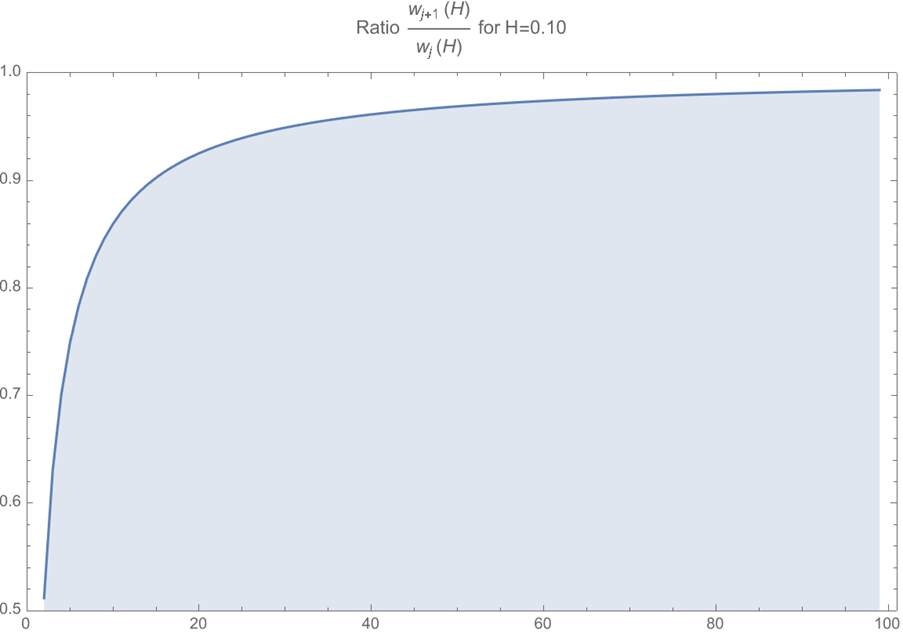
What does this mean in practice? If the weights are so close (and small) as to be (almost) interchangeable and you need a lot of them (the original Rough Volatility paper uses 500 lags), one could sample the historical distribution (or use its summary statistics) to predict not only the expected value of the next volatility, but also the dispersion of the volatility. And having a good idea of this dispersion is really useful, even if it is to establish that this uncertainty is such an integral part of volatility that it explains well why it is so hard to be sure of a trend – it is very hard to rule out volatile volatilities.
More details about Rough Volatility can be found at the Rough Volatility Network. My upcoming thesis will discuss Hawkes processes and volatility inference in more detail.
Marcos Costa Santos Carreira is a PhD Candidate at École Polytechnique. His article was first published in the QuantMinds eMagazine.