Optimal VaR adaptation in transient environments

Volatility spikes during the early phase of the pandemic in 2020 have once again highlighted weaknesses of traditional Value at Risk (VaR) estimates when it comes to changes in financial market environments. Although potential remedies have been available for some time, the concrete implementation of solutions in running VaR systems seems to be more challenging.
During the first half of 2020, many banks experienced large numbers of backtest outliers when they compared actual profit and loss numbers to VaR estimates in the trading book. The simple reason was that their regulatory VaR systems were not able to adapt to rapidly changing market conditions as volatility spiked to ever-higher levels. The problem lies with the amount of data that is used to “train” the VaR system.
In a nutshell, this amount of data is a compromise between having enough observations to compute relevant statistical quantities (here we want lots of data) and the degree to which this data is still relevant for the current environment (here we only want recent data). Whereas in quiet times collecting large amounts of data to reduce measurement uncertainty seems to be a priority in some model risk management approaches, the situation changes once there is a rapid shift as experienced in March 2020. Obviously, this may call for some mechanism to “learn” how to spot a crisis environment – but for now, a simpler approach may already deliver some benefits.
The situation can be formalised by looking at a noisy random walk, i.e. a stochastic process with identical and independent innovations for which we have observations that include some additional disturbances. The important thing to notice is the existence of two distinct sources of randomness, the innovations and the disturbances. It is clear that in calm times, innovations are the minor term and collecting large amounts of data will help. However, whenever the innovation term is not negligible any more – as at the beginning of some transient market environment – recent observations will contain much more information.
Usually – and this solution has been around for decades – one attaches weights like in a GARCH time series framework. However, in practice there are considerable difficulties in deriving the optimal decay parameters. Sometimes there is a considerable calibration instability due to maximum likelihood derivations and the only help is using the classical RiskMetrics decay parameters.
A straightforward alternative would be to use a simple state space approach and treat the unperturbed random walk as a hidden state for which we have noisy observations. This will lead to some very easy optimality criterion that only depends on the Signal to Noise Ratio (snr). In this case, the Signal to Noise Ratio is the ratio between the variance of the innovation term and the variance of the disturbance term. The decay parameter would then be given as
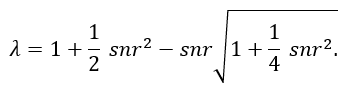
One can see the crucial effect of the Signal to Noise Ratio; low values of snr indicate calm times in which there is no need to pronounce recent observations. As values for snr increase, the decay parameter decreases and therefore recent observations yield a much bigger influence in estimating the current (volatility) state.
That approach is easily extended to include auto-regressive time series models instead of random walks; in this case, the optimality criterion can also be derived analytically. Nevertheless, where does this leave us when it comes to improve current VaR systems? Let us assume that we have a scenario based VaR system that has difficulties in adapting to current market conditions such as a situation of increased volatility.
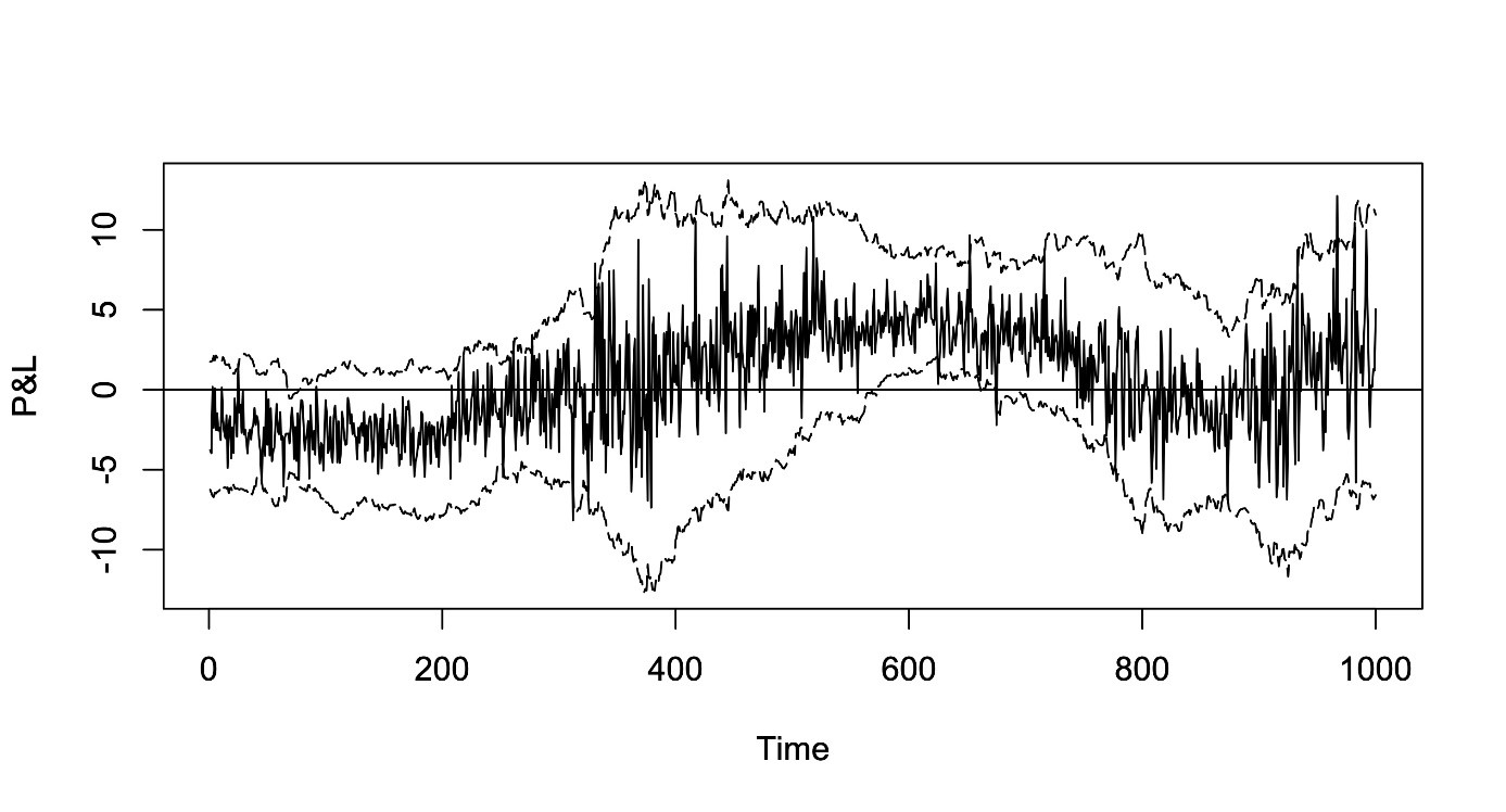
In this case, we could combine the aforementioned state space approach and rescale all scenarios of the VaR calculation based on corresponding local drift / variance estimates. The following diagram shows the case of an example from a Monte Carlo benchmark exercise. Even though there is a considerable innovation in the drift as well as the variance process, the relatively simple rescaling approach yields a quite good performance in tracking the profit and loss profile. Of course, such a location / scale correction will not account for deficiencies of the VaR system with respect to tail events.
How to use these aspects within a risk model validation framework? One can easily integrate such improved VaR calculations into the context of benchmark exercises. Banks using internal models under Pillar 1 already know the concept of “Stressed VaR”. Based on the previous remarks it is easy to analyse the behaviour of different VaR models during the transition from a normal period into the stressed period and back again. More details as well as additional Monte Carlo Studies can be found in the third edition of the book on Risk Model Validation by my colleague Christian Meyer and me. Adaptation of VaR systems will also be the topic of my talk at QuantMinds late May 2021. Contact peter.quell@dzbank.de.