Optimising variable annuity reserves through deep hedging

 Deep hedging is a new machine learning technique that delivers a more efficient strategy for hedging market risks than traditional risk neutral pricing. Risk neutral pricing has been the basis for most derivatives pricing over the last fifty years, but the suite of assumptions it makes about markets and the hedging problem often fail in practice. Deep hedging matches the risk neutral limit when appropriate, but also provides a quantitative framework for improving upon it when those risk neutral assumptions are violated.
Variable annuity reserve calculations are exactly one of these scenarios. The reserve that an insurer needs to hold can be materially reduced by using deep hedging to define a rules-based hedging strategy, which at the same time avoids the computational complexity of the “nested stochastics” problem that insurers encounter when applying risk neutral hedging to this calculation.
Life insurers can use Beacon’s deep learning analytics coupled with policy data and large-scale elastic cloud compute to experiment with and implement this technique at enterprise scale, reducing their reserves and increasing their return on equity.
What are variable annuities?
Variable annuities are a popular investment vehicle sold by life insurance companies, where an investor puts money into an equity fund, receives tax-deferred gains, and receives the proceeds after retirement as an annuity.
The life insurer that issues a variable annuity has a somewhat complex liability: such policies are commonly issued with a “guaranteed minimum death benefit” such that if the investor dies before annuitisation, their beneficiaries receive the present investment account value floored at a guaranteed minimum, often the principal investment. If the account value is less than this floor, the insurer is liable to pay the difference to the beneficiary; that difference looks like the payoff of an equity put option. In return for that guarantee, the insurer receives a fee paid by the investor while alive.
There are many different flavours of variable annuity with more complex terms, but this simple example highlights the main risk in these products: the insurer is short equity put options, often with quite long maturities, which are conditioned on realised mortality.
Variable annuity reserves and the lifetime PNL distribution
Insurance regulators require insurers to hold a reserve against their variable annuity liabilities. That reserve calculation is complex but can be approximated as the 70%-ile expected shortfall of the lifetime PNL (profit-and-loss) distribution of the variable annuity portfolio: that is, the expected loss conditioned on the loss being larger than the 70%-ile value at risk.
This lifetime PNL distribution is generated through a Monte Carlo simulation of market factors. That simulation is in the “real world” probability measure, as opposed to the risk neutral probability measure, which means that average equity returns are set to historically observed returns (normally 8-9%/year) rather than the risk-free rate.
Insurers are allowed, if they choose, to include a rules-based hedging strategy which also contributes to the lifetime PNL distribution. Including hedges will tend to reduce the standard deviation of that PNL distribution. They can also choose not to incorporate a hedging strategy into their reserve calculation. Note that this choice does not affect whether the insurer actually hedges their position in practice, just whether they include a hedging strategy in their reserve calculation.
---
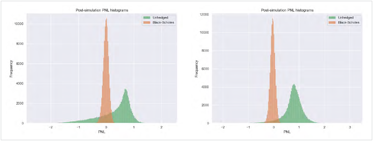 Figures 1 and 2: histograms of the lifetime PNL distribution of a variable annuity portfolio. Figure 1, on the left, is for an average equity return of 5%, and Figure 2, on the right, is for an average return of 15%. The orange distribution is the “hedged” distribution, where at every point the variable annuity portfolio is hedged with risk neutral hedges. The green distribution is the “unhedged” distribution where no hedges are ever applied. In Figure 1 the 70%-ile expected shortfall is larger for the unhedged distribution than for the hedged distribution, and the reserve is smaller when the hedging strategy is included in the reserve calculation. In Figure 2 the opposite is true: the insurer will see a smaller reserve if they exclude the risk neutral hedging strategy in their reserve calculation.
---
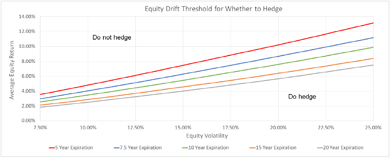 Figure 3: the hedging threshold as a function of average equity return, equity volatility, and time to expiration of the variable annuity portfolio. For example, the red line shows the threshold for a 5y expiration; if the average equity return is above the red line, it is better for an insurer not to include risk neutral hedges in their reserve calculation; if the average return is below the red line, it is better to include the hedges. This is calculated for a simple geometric Brownian motion model of the underlying equity with a constant average return and volatility.
---
However, because these simulations may use relatively high average equity returns, and because the insurer is long equities (through selling equity put options), the mean of the unhedged PNL distribution can be far enough to the right to make the reserve, equal to the 70%-ile expected shortfall, smaller for the fully unhedged PNL distribution than for the distribution that includes hedges.
In addition, incorporating hedges into the reserve calculation can be computationally very expensive. Hedge notionals must be calculated at each timestep and for each path of the Monte Carlo simulation. The calculation of those hedge notionals involves calculating the price of the remaining variable annuity portfolio, which itself generally requires its own Monte Carlo simulation. This is the “nested stochastics”, or “stochastics on stochastics”, problem and means that in practice many insurers cannot practically calculate a reserve that incorporates a hedging strategy.
For these two reasons – nested stochastics, and that the calculated reserve for the unhedged distribution can be less than the reserve from the fully-hedged distribution – many insurers do not include a rules-based hedging strategy when reserving for their variable annuity liabilities.
Deep hedging delivers a hedging strategy that minimises the reserve, automatically under-hedging if the average equity return is high enough. And the hedge notionals at each timestep are calculated through a cheap neural network evaluation rather than an expensive Monte Carlo simulation, so do not suffer from the nested stochastics problem.
Deep hedging: Improving on risk neutral pricing
Risk neutral pricing has been the foundation for derivatives pricing and risk calculations since the introduction of the Black-Scholes model in the early 1970s and includes all the standard extensions of that model to stochastic and local volatility, multi-factor curve models for interest rate and commodity forward curves, and much more. It has been a remarkably successful framework for managing the market risk of complex derivative portfolios.
It rests on several main assumptions:
- There are no unhedgeable risks.
- There are no transaction costs or liquidity constraints associated with hedge trades.
- Hedging is continuous – that is, hedges are dynamically rebalanced continuously as markets move and risks change.
When these assumptions are satisfied, the lifetime PNL after hedging a derivatives portfolio is certain because all the risk is hedged away. The lifetime PNL distribution in that case is a delta function: a spike at one specific value. The fair upfront premium for a derivative is set such that this certain lifetime PNL is exactly zero.
In practice, all these assumptions are violated in one way or another in real markets, and the lifetime PNL distribution is spread out since there is residual unhedged risk. Investor risk preferences then come into play.
Deep hedging, introduced in a 2018 paper, describes a quantitative method to price and hedge derivatives when those risk neutral assumptions are violated. It does this by replacing the risk neutral hedge calculation with a trainable non-linear function – a neural network. The neural network is trained to minimise a convex risk measure of that lifetime PNL distribution. A standard example of a convex risk measure is expected shortfall: the expected loss if the loss is greater than the value at risk. The expected shortfall of a distribution incorporates both the mean of that distribution as well as its spread.
After training, deep hedging delivers a function that takes in the current market state and portfolio information and returns the optimal hedges to trade. If that hedging strategy is followed, and markets evolve statistically as assumed, then the expected shortfall will be minimised over the life of the portfolio. Crucially, that function is quick to calculate: a neural network evaluation consists predominantly of linear algebra for which modern neural network packages easily take advantage of hardware architectures across multiple CPUs and GPUs.
Deep hedging reproduces the risk neutral hedging strategy in the limit that the risk neutral assumptions are satisfied, but also does better: when those assumptions are violated it gives a quantitatively better hedging strategy for the goal of minimising the expected shortfall of the lifetime PNL distribution.
Deep hedging and variable annuity reserves
In the preceding discussion, it was assumed that the inclusion of a rule-based hedging strategy in the reserve calculation came down to an all or nothing decision: do not hedge at all or hedge all the time using the risk neutral hedges.
Deep hedging gives insurers another option. When the neural network is trained to deliver hedges that minimise the 70%-ile expected shortfall of the post-hedge lifetime PNL distribution, it learns not to hedge at all when average equity returns are well above the threshold as portrayed in Figure 3, and hedges comparably to risk neutral hedges for average returns well below the threshold. Plus, it gives a quantitative metric for smoothly varying from one to the other for average returns near the threshold.
As an example, consider the case of 8% average equity return, 20% volatility, 1% mortality rate, and 5 years’ term on the insurer’s liability on $100 of initial assets under management. In this case, the deep hedger learns to materially under-hedge in comparison with risk neutral hedges but does not leave the variable annuity position completely unhedged. This results in a 70%-ile expected shortfall of close to zero, less than both the unhedged PNL distribution and the PNL distribution using risk neutral hedges.
In this simplified example, the reserve calculated from the scenario-based simulation would be almost zero.
---
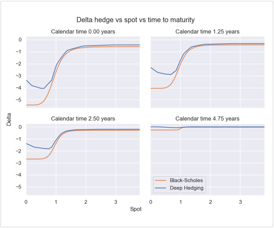 Figure 4: hedge notional (on the y-axis) as a function of equity price (on the x-axis, as a ratio to initial equity price) for an 8% average equity return and 20% volatility, for four calendar times: 0 years, 1.25 years, 2.5 years, and 4.75y (the last only 0.25y before the end of the term). The orange lines show the risk neutral hedge notional, which is traditionally what an insurer would include as a rules-based hedging strategy in their reserve calculation. The blue lines show the deep hedger hedges, which materially under-hedge compared to the risk neutral strategy, so that the post-hedges distribution can take advantage of the positive average equity return while short equity.
---
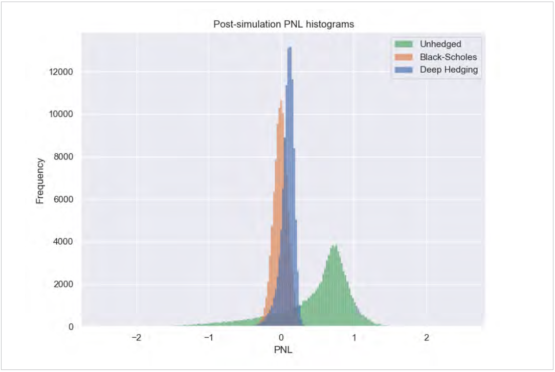 Figure 5: lifetime PNL distributions for three cases for an 8% average equity return: unhedged (green); hedged with risk neutral hedges (orange); and hedged with deep hedger hedges (blue). The 70%-ile expected shortfall is larger for the risk neutral hedge scenario than for the unhedged scenario, so traditional hedging approaches would suggest that insurer not include a rules-based hedging strategy in the reserve calculation. However, the 70%-ile expected shortfall of the deep hedger scenario is close to zero, eliminating this scenario-based reserve if this rules-based hedging strategy were incorporated in the reserve calculation.
---
Notice that the deep hedger under-hedges more aggressively when equity price is low. These cases correspond generally to more negative PNL outcomes where running a larger net risk position allows the insurer to take advantage of the positive (real-world) average equity return to shift PNL up over time. When equity price is high, on the other hand, a positive PNL is more locked in, and the deep hedger hedges more aggressively, converging to the risk neutral hedging strategy.
Beacon and deep hedging
Beacon is at the forefront of deep hedging research because we see it as a valuable technique for clients, like life insurers, to improve business performance through analytics run at enterprise scale.
Implementing a robust deep hedging-based reserve calculation in production requires a number of elements:
- Variable annuity policy data. Easy access to the full set of policies through a modern data warehouse lets actuaries, quants, and data scientists build complex and reliable analytics.
- Actuarial model data. Like policy data, reliable mortality tables and related information should be close at hand to make it easy to build new analytics that depend on them.
- Market data. Reserve calculations depend on equity and interest rate market data for levels, volatilities, and correlations.
- Derivatives analytics. Variable annuity hedges are often complex financial derivatives such as futures, options, and more exotic derivatives such as cliquets and basket options.
- Machine learning analytics. Deep hedging is one of the first applications of real machine learning to front office pricing and risk problems and requires modern machine learning tools to execute efficiently.
- Compute infrastructure. Running large-scale Monte Carlo simulations on large variable annuity portfolios is computationally expensive even without the nested stochastics problem. Executing these calculations robustly requires significant grid compute, ideally rented from the cloud so you pay for as much compute as you need, only when you need it.
- Reporting tools. The results of the reserve calculations need to be reported to the finance team and to management in a robust way with ability to slice and dice the results to evaluate the details.
Beacon’s enterprise technology platform products have all these components, organised end-to-end to help actuaries, quants, and data scientists experiment at scale and deliver value to their business quickly while still satisfying enterprise controls.
Conclusions
Deep hedging is an exciting new technique in derivatives risk management, and in this white paper we applied it to optimising reserves for a variable annuity portfolio.
There are three key insights from this analysis:
- When average equity returns are near or above a threshold, deep hedging delivers an under-hedging strategy that balances risk reduction with being long the market in a way that substantially reduces reserves compared to either not hedging at all or hedging entirely with risk neutral hedges.
- Deep hedging avoids the “nested stochastics” problem that makes incorporating risk neutral hedges computationally infeasible in many cases.
- Managing variable annuities requires enterprise-scale technology, and an integrated data and analytics platform like Beacon’s makes it easier to test and deploy new techniques like deep hedging that can materially improve a life insurer’s return on equity.
In the end, this technique allows life insurers to hold smaller reserves against existing variable annuity portfolios and attain higher returns on equity.

About Beacon
Beacon is a cloud-based platform designed to empower developers, quants, data scientists and business users to scale technology and achieve their business goals. Beacon is the only vendor who gives clients the underlying source code, a developer platform, and infrastructure services so that clients can own the full technology stack. The Beacon platform will enable corporate innovation and fit your business needs today, tomorrow and in the future.
Beacon was founded in 2014 by the senior technologists who worked with SecDB at Goldman Sachs and created Athena at JP Morgan and Quartz at Bank of America Merrill Lynch. Beacon has over 70 employees with offices in New York, London and Tokyo.
Web: www.beacon.io
E-Mail: info@beacon.io