Rebalancing portfolios with crash/rally indicators

In today’s turbulent market conditions, how do you determine your investment strategy? How do you make the most of all the assets in your portfolio? Prof Dr Jerome L Kreuser, Senior Researcher, Department of Management, Technology and Economics, Zürich Switzerland and CEO and Founder of RisKontroller Global LLC, uses crash/rally indicators to inform his decisions.

In our last article, we discussed our crash/rally methodology, which we call Efficient Crashes Optimizer (ECO)[1], including the equations of our model. We showed how we can we predict crashes and rallies with a probability better than chance. In this article, we will convert theory into actionable information to go beyond a simple prediction to enhance trading performance and amplify alpha.

We first review some terminology of our model we presented before. Then we discuss information generated from the model and how to use and apply that information.

We define the following set of variables:

Δt	= discrete time interval [t, t+1]
pt	= price of the risky asset at time t
	= expected return of the risky asset on Δt when there is no crash or rally
σ	= standard deviation on Δt of the geometric random walk price process
εt	= sample from a standard normal distribution at time t
rD	= discount rate of the asset price on Δt
rN	= growth rate of the “normal price” on Δt
rf	= risk-free rate on Δt
p0	= starting price of the risky asset
Nt	= p0exp(rNt) : this defines the normal price process
ρt	= probability that there is a correction (crash or rally) at time t
	= the size of the ith corrective jump relative to the distance to the normal price. We refer to it as the “crash factor”
ηi	= probability that, when there is a correction, it is of size Ki
	= expected corrective crash size relative to the distance to the normal price or expected crash factor
	= the relative (negative) mispricing of the risky asset

We introduce the simple stochastic price process with a discrete Poisson process.

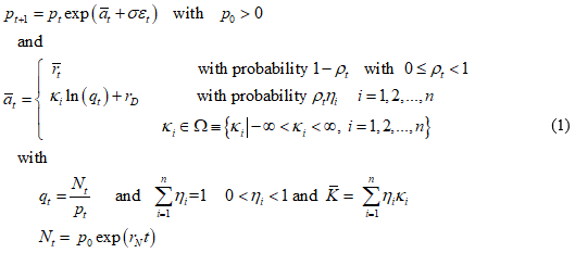
At each time step, there is a probability ρ_t for a crash/rally to happen with an amplitude that is proportional to the bubble size, or amplitude defined as  where and r_N is defined as the long-term average return^[2].

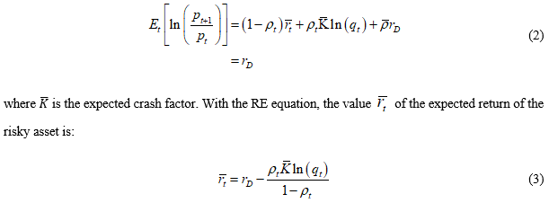
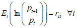We assume that the expected return  is determined in accordance with the Rational Expectation condition which reads

We form a Kelly (expected log of wealth) problem. Let λ_t be the fraction of wealth W_t allocated to the risky asset in time t and 1-λ_t the allocation to the risk-free asset with return r_f. Then

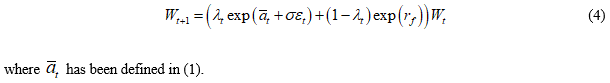
We wish to determine

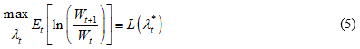
where E_t is the expectation conditional on the information up to time t.[3]

We discuss here the implementation of our methodology in simple terms to a portfolio and in further articles we will extend it to general portfolio models including dynamic stochastic optimisation models. The two important points here are that the method extends classical Kelly to the case of GBM plus jumps in the context of our RE bubble model and that the results applying equation 5 are useful and applicable even if there is no crash or rally.

Obtaining actionable information

In Table 1 we illustrate some of the output (generated on 1 May 2019 and evaluated on 1 June 2019) from the model[4], where:

• Ex return is the expected return  adjusted for one month.
• Size is the size of the predicted crash or rally,   adjusted for one month. Size > 0 is a rally and < 0 is a crash.
• Hedge is the value of λ_t
• Prob is the value of ρ_t
• Return no crash is the value of 
• Prob trend is the change in the probability as a percent
• Predicted return w hedge is the return predicted if the hedge had been made
• Actual return w hedge is the actual return over the month of May if the hedge had been taken
• Actual return is the actual return the asset obtained over the month of May

The last row is all averages. Therefore, the last column gives the actual return on an equally weighted portfolio of -0.93% for the month of May. If each asset were to be hedged individually, the return on an equally weighted portfolio of such assets would be 0.60%.

The hedged asset return is obtained by taking λ_r + (1-λ)r_f with r the expected return or the real return on the asset and r_f the return on the risk-free asset here taken to be 2.5% annualised.

The method did not do well on equities for May 2019. The Russell2000 had almost a 60% chance to jump up by almost 12%. It didn’t happen. In fact, equities were down across most classes primarily due to tariff threats that were not priced into the data and so were not identified by the model. Overall, the use of the ECO method improved returns by 1.53% for the one month of May.

With this simple information, here is a list of output values you could review on an asset by asset basis:

1. The size and sign of the expected return.
2. The size of the hedge. With a value closer to 2 it has a chance to be a good bet, whereas with a value close to -1, the risk-free asset is a better bet.
3. The relative value of the size of the crash/rally and associated probability relative to the return with no crash as an indicator of volatility.
4. The probability trend. Is the probability of a crash/rally increasing or decreasing?
5. The average expected return and average hedge give an overall picture of the expected direction of asset movements.

The optimal way to invest using the method discussed in Kreuser and Sornette, 2018, is to take the hedge. But this takes no account of the context within a portfolio. We will discuss the portfolio context in a forthcoming paper.

These criteria worked well for some assets and less well for others. It would not have worked well for Russell2000TR but would have for Australia Stocks. It worked well for the assets highlighted in green. Especially well for NatGas where the expected return almost matched the actual return and the predicted return with the hedge almost matched the actual return with the hedge.

Extracting information from dynamic probabilities

The probability ρ_t is computed by measuring the probability of jumps on a window of historical price data. We follow the basics of Jacquier and Okou (2014) in order to do that.

However, the probability of a crash or rally will increase whenever the prices accelerate upward for a crash or downward for a rally (Xiong and Ibbotson, 2015 and Ardila-Alvarez et al., 2016). This was most notably observed in the Bitcoin bubble[5].

If we could measure the acceleration
we could compute ρ_t directly from equation (3) as we assume we know the other variables (Kreuser & Sornette, 2018a). We call this the dynamic probability.

In Figure 1, we see the graph of the Bitcoin price overlaid with the normal price and the value of the hedge parameter λ_t. There are two important points in this graph. First, you can see how the Bitcoin price is accelerating, and second, you can see how the value of λ_t is going to zero. It becomes zero on 19 Dec. 2017.

We see some of the data output from the ECO method in Table 2 leading up to 19 Dec. 2017. Besides λ_t going to zero, we see the asset price accelerating and the dynamic probability increasing to 0.78. After the 26 Sep. 2017 the historically estimated probability of a crash was dominated by the dynamic probability. We even calculated the size of the crash using very accurately. The results were posted on LinkedIn on 21 Dec. 2017 and sent to an FT editor on that date. Details are in Kreuser & Sornette, 2018a.

The dynamic probability and related values are stochastic indicators of a crash/rally. See the short-term Bitcoin price in 2017 in Figure 2 and you will see that the acceleration is unsustainable. We can probabilistically quantify the probability of the crash, the size, and the timing using the ECO method.

Portfolio marginal rebalancing

We will discuss integrating the ECO model into other portfolio models in subsequent QuantMinds articles. But in this section, we discuss how using the same outputs can generate what we call a Zero-sum Support Vector (Support Vector). Suppose we want to rebalance only a small percentage of the portfolio; for example, x%. We want to associate with each asset a percentage to be bought (>0) or sold (<0) so that the total sums to zero. Then purchases are funded from sales. We don’t consider transaction costs here, but they would be easy to add.

In Table 3, we see additional outputs from the method, where:

• Outper is the estimated outperformance
• Reliability is a factor indicating the reliability of the results based on outperformance
• Actual returns % is the actual return of the asset for the month of May
• Zero sum Alloc. is the calculation of the zero-sum Support Vector
• Support Percent alloc. is the zero-sum Support Vector expressed as percentages with actual returns
• Support return % is the actual percent return on the Support Vector for each asset and the total

The last column gives the return for each asset using the computed Support Vector percentages in the column before the last one (Support Percent alloc.).

The Support Vector is a strategic tilting of the portfolio for whatever percentage of it is desired.

The column labled Outper gives the outperformance of the method using a historical window. The parameters r_D and r_N are estimated by fitting an exponential without anchoring to a short and long window respectively of historical prices. The window of time between rebalancing is selected to be of a number of days. Combinations of these parameters are examined and the combination that gives the best outperformance of the Efficent Crashes Portfolio (combination of risky asset and risk-free asset) over the risky asset are used for the estimations at the current time. The higher the outperfromance, the better is the assumed estimation for the current time.

The Reliability column scales the outperformance to be between 0 and 10 and assumes the higher values give more reliable results than the smaller values.

The column labeled Zero sum alloc. computes the raw numbers for calculating the percentages for the Support Vector. The computation is done in the following way:

Let a_i represent the marginal return on one unit of asset i. Let x_i represent the number of units of asset i acquired. Let us assume that the marginals are such that which can be positive or negative. Let us put a limit on the amount that can be acquired as it may otherwise be infinite. We express that limit as Then we wish to solve the problem of adjusting a portfolio to maximise the marginal return as:

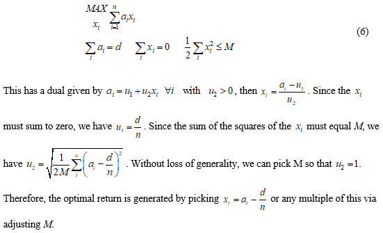
We take a_i to be the absolute value of the expected return (Column 1 of Table 1) times the hedge (Column 3 of Table 1) as this is the amount of the asset you would use in ECO. Thus, the x_i are the respective asset allocations. These are scaled to percentages in the column Support percent alloc. Then the last column gives the respective returns for each asset and if the portfolio is rebalanced in the percentages indicated by the Support Vector, you would have obtained a return of 1.81% for however much you chose to rebalance.

Comments and summary

The examples used here have been chosen for illustrative purposes. There is no guarantee of a positive outcome. However, in extensive experiments[6] and on many real applications including with a large fund, we have been successful enough to conclude that the method performs very well. Furthermore, our method behaves as an extension of Kelly to prices that satisfy Geometric Brownian Motion with jumps, where jumps are relative to a normal price process, which is different from the method discussed in Davis and Lleo, 2015.

Even if there are no significant jumps and we are not on the verge of a crash or rally, the method generates useful information used to rebalance a portfolio even at the margin.

The reader may have noticed that -1≤ λ_t ≤2. We bound it in this way to prevent more extreme movements in the Efficient Crashes portfolio. For a similar reason, you would use fractional Kelly in the classical Kelly method.

The Support Vector is designed to be independent of the current asset allocation. The Support Vector gives adjusted allocations that we can express in percentages of an amount rebalanced such that the total percentages sum to zero. Therefore, the negative values represent amounts sold and the positive values amounts bought. It can be considered as an augmented application in support of an inhouse risk management system. We may think of the Support Vector as a strategic tilting of the portfolio for however much is desired.

We have not included jump dependencies in the computations here. We intend to do that in a forthcoming article.

References

Ardila-Alvarez, Diego, Zalan Forro, and Didier Sornette. 2016. The Acceleration Effect and Gamma Factor in Asset Pricing, Swiss Finance Institute Research Paper No. 15-30. Available at SSRN: http://ssrn.com/abstract=2645882.

Davis, Mark H. A., and Sebastien Lleo. 2015. Risk-Sensitive Investment Management. Singapore:World Scientific Publishing.

Sornette, D. and P. Cauwels. 2015. “Financial bubbles: mechanisms and diagnostics”, Review of Behavioral Economics 2 (3), 279-305. See https://www.ethz.ch/content/specialinterest/mtec/chair-of-entrepreneurial-risks/en/financial-crisis-observatory.html

Jacquier, Eric and Cedric Okou. 2014. “Disentangling Continuous Volatility from Jumps in Long-Run Risk-Return Relationships”, Journal of Financial Econometrics 12 (3), 544-583.

Kreuser, J. and D. Sornette. 2018a. “Super-Exponential RE Bubble model with efficient crashes”, The European Journal of Finance, Volume 25, 2019 – Issue 4. Also see http://riskontroller.com/ and https://papers.ssrn.com/sol3/papers.cfm?abstract_id=3064668.

Kreuser, J. and D. Sornette. 2018b. “Bitcoin Bubble Trouble”, Wilmott Magazine, May, and at SSRN https://papers.ssrn.com/sol3/papers.cfm?abstract_id=3143750.

Merton, Robert C. 1980. “On Estimating the Expected Return on the Market.” Journal of Financial Economics 8: 323–361.

Xiong, James X., and Roger Ibbotson. 2015. “Momentum, Acceleration, and Reversal.” Journal of Investment Management 13 (1): 1st quarter.

Ziemba, William T.; Sebastien Lleo; and Mikhail Zhitlukhin. 2018. “Stock Market Crashes”, World Scientific Series in Finance, Vol. 13.

Notes

[1] The term “Efficient Crashes” is taken from the Kreuser & Sornette, 2018a, paper.

[2] We call it the “normal price return”. Some may interpret this as a fundamental price return but that is not the specific intention here.

[3] For more details see the previously referenced article or the paper Kreuser, Jérôme and Didier Sornette (2018). “Super-Exponential RE Bubble Model with Efficient Crashes”, The European Journal of Finance, Volume 25, 2019 – Issue 4. Also see http://riskontroller.com/ and https://papers.ssrn.com/sol3/papers.cfm?abstract_id=3064668 .

[4] The data is a subset of the data used in our AugurMax portfolio and reported on at http://riskontroller.com/investible-universe/ .

[5] Kreuser, Jérôme and Didier Sornette (2018b). “Bitcoin Bubble Trouble”, Wilmott Magazine, May.

[6] We are currently completing a simulation study with ETH Zürich.