The convexity profile of systematic strategies and diversification benefits of trend-following strategies

How do you measure your investment strategy’s risk-adjusted performance? Artur Sepp, Director of Research at Quantica Capital AG, uses regime conditional model to analyse the convexity profile of quantitative strategies and hedge funds.

We introduce regime-conditional regression model to measure the risk profile of systematic investment strategies. We apply this model to classify systematic strategies into defensive and risk-seeking strategies with either positive or negative risk-premia alpha. We show that trend-following CTAs belong to an exemplary class of defensive active strategies with insignificant risk-premia alpha. As a result, the trend-following CTAs provide a valuable diversification benefits for balanced and alternative portfolios.

Risk profile of investment strategies

Quantitative strategies can be characterised by the convexity of their returns that measures how strategies behave in tail events. Using realised returns, we can evaluate the convexity in a few ways.

1. Skewness coefficient measures the asymmetry of strategy returns. Negative skewness indicates higher downside risk (see 1).
2. Quadratic convexity (see 2) measures the convexity of a strategy relative to its benchmark, such as equity market index.
3. Regime conditional betas (see 3) evaluate linear regression betas of a strategy conditional on the bear/normal/bull periods of its benchmark.

Regime conditional betas

We introduce a locally linear regression which approximates the quadratic or polynomial profile of quantitative strategies applied in the following way (see 3 for more details). First, we select a benchmark to analyse the performance of a strategy relative to this benchmark, as in case for the quadratic regression. In the following examples, we choose the S&P 500 total return index. We specify the return frequency with non-overlapping periods (monthly, quarterly) and compute paired returns of the strategy and its benchmark. Then we sort the pairs by returns on the equity index. After the sorting, we label returns of the benchmark that are below the 16% quantile, which approximately corresponds to returns below one standard deviation, as belonging to the bear regime. In a symmetric way, we label returns above the 84% quantile, which correspond to returns above one standard deviation, as belonging to the bull market regime. Finally, we label returns in the middle (returns approximately within one standard deviation) as belonging to the normal regime. The empirical frequency of bear, normal, and bull regimes is 16%, 68%, and 16%, respectively.

In the Figure 1, we illustrate the linear, quadratic, and regime-conditional regressions for the SG trend index, which benchmarks the performance of large CTAs managers with the focus on trend-following strategies. We apply the S&P 500 total return index as the equity benchmark.

1. The quadratic regression has a large positive estimate of the quadratic convexity. This indicates that the SG Index benefits from large returns of the benchmark index on both downside and upside.
2. The regime conditional regression illustrates how the profile of the SG Index changes relative to the equity benchmark. In bear regimes, the SG index has a strong negative equity beta, so the SG index provides the downside protection for falling equity markets. In bull regimes, the SG index has a positive equity beta so that it participates in the upside of equity markets.
3. Notably, the linear regression implies a negative beta for the SG index, yet it underestimates the diversification benefit in the bear regime by a factor of 3 compared to the regime conditional and quadratic regressions. This observation highlights how important it is to account for non-linear profile of systematic strategies.

We see that the regime-conditional model can be interpreted as a local approximation to the quadratic regression. Yet it is relatively easy to explain the regime-conditional model and its implications for the regime-conditional risk profile. For an example, a -10% loss on the equity index implies a gain of +6% on the SG Trend index. It is a bit more complicated to compute the same inference for the quadratic model without relying on a calculator. We recall the famous quote by Einstein: “Everything should be as simple as it can be, but not simpler”.

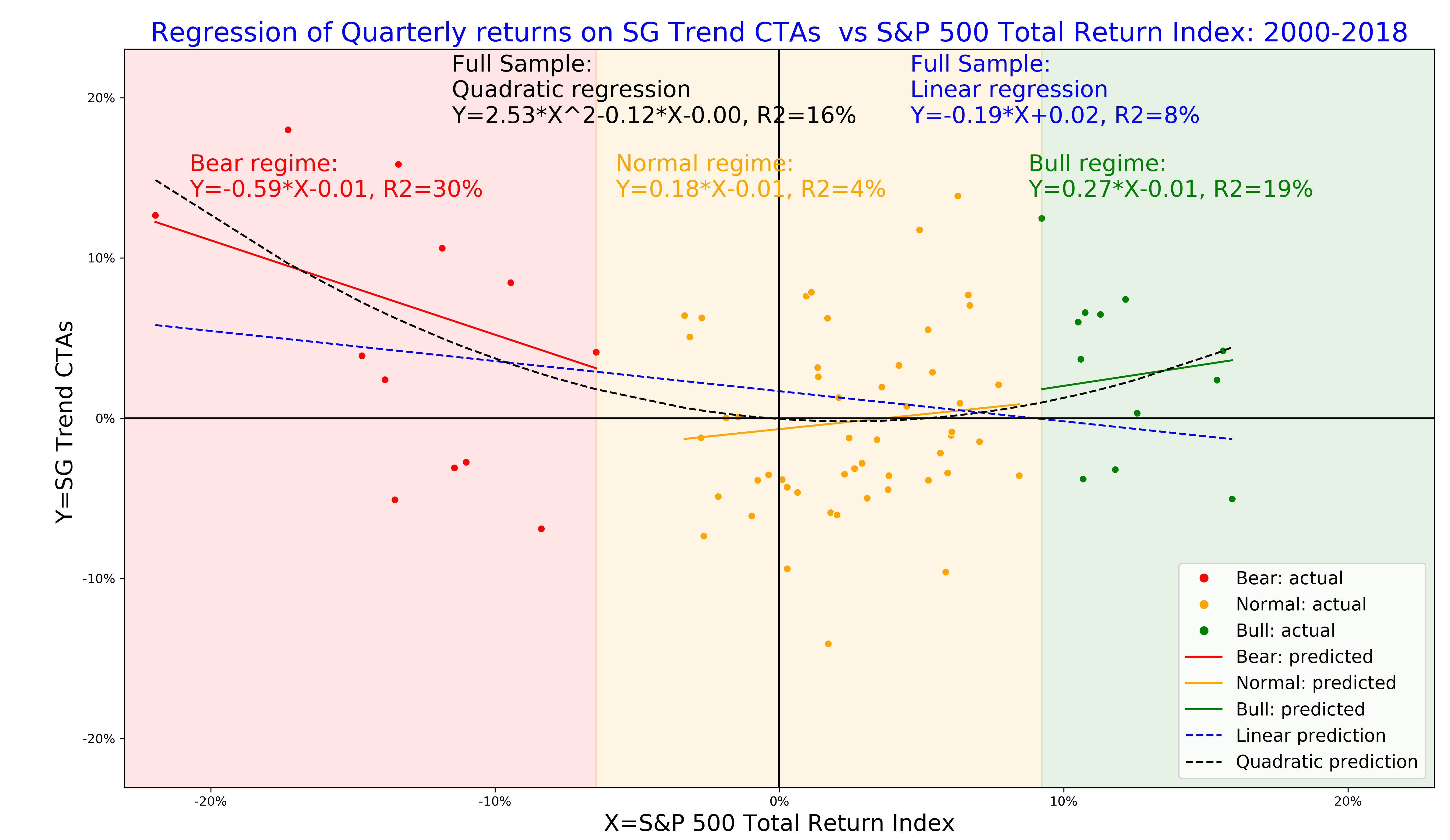
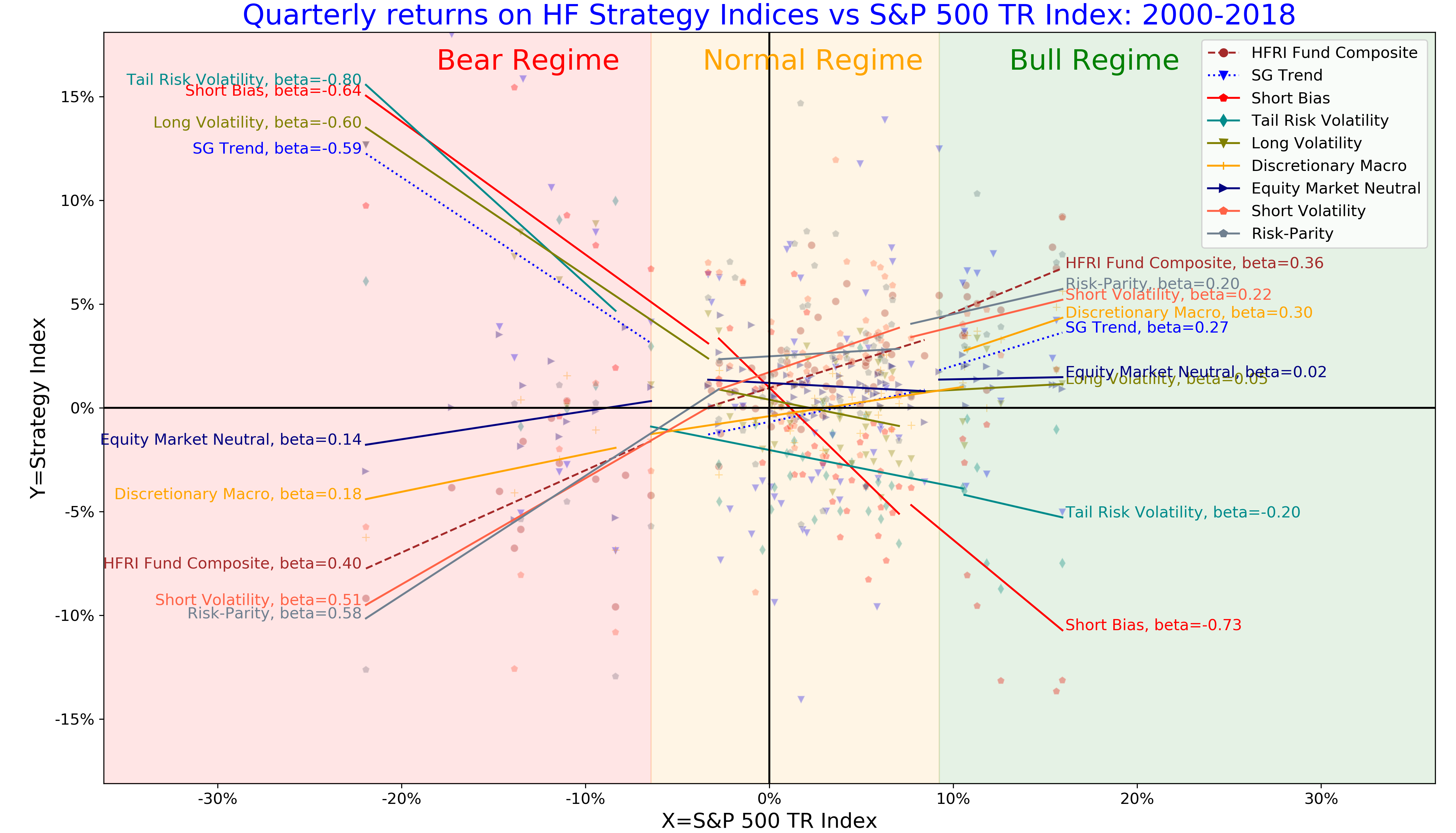
Convexity profile of hedge fund strategies

We apply the regime conditional regression to analyse the convexity profile of hedge style indices. In Figure 2 we illustrate regime conditional betas for a selection of hedge fund style from HFR indices data using the S&P 500 index as the equity benchmark.

We can classify the strategies into defensive and risk-seeking based on their return profile in bear regimes:

1. Defensive strategies have negative equity betas in bear regime so that these strategies serve as diversifiers of the equity downside risk.
2. Risk-seeking strategies have positive marginal betas in bear regime. Equity betas of most of risk-seeking strategies are relatively small in normal and bull periods but equity betas increase significantly in bear regimes. Most notable examples include short volatility and risk-parity strategies. We term these strategies as risk-seeking risk-premia strategies.
3. We term strategies with insignificant betas in normal bear regimes as diversifying strategies. Examples include equity market neutral and discretionary macro strategies because, even though these strategies have positive betas to the downside, the beta profile does not change significantly between normal and bear regimes. As a result, the marginal increase in beta exposure between normal and bear periods is insignificant.

Further, we observe an interesting pattern for the defensive strategies.

1. Short bias, long, volatility, and tail risk volatility strategies represent defensive strategies with a systematic negative equity bias. These strategies either short equity markets consistently or buy protective options without delta-hedging. We term these strategies as defensive short risk-premia strategies because of their systematic short bias.
2. Trend-following CTAs are termed as defensive active strategies because these strategies deliver down-side protection but unlike short risk-premia strategies do not have a systematic exposure to shorting risk-premia, for example, either through buying options or credit protection. In contrast to defensive short risk-premia strategies, trend-following CTAs deliver positive betas in normal and bull regimes by actively managing their exposures.

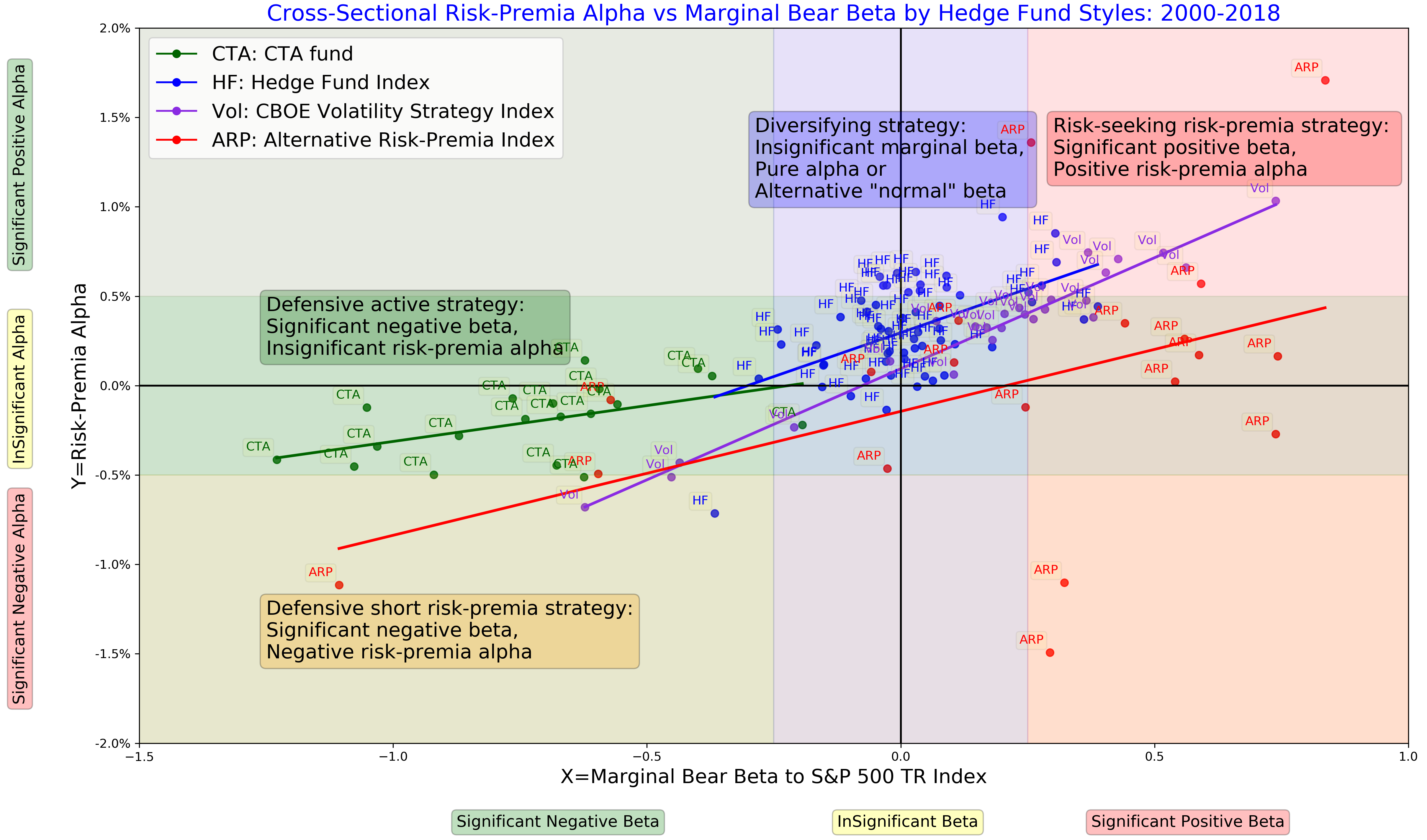
Risk-premia alpha as compensation for the tail risk

Finally, we address an important question whether a strategy delivers an appropriate compensation for taking risk exposures. To answer this question, we define the risk-premia alpha as the intercept of the regime-conditional regression model for strategy returns regressed by returns on the index.

We apply the cross-sectional analysis of risk premia for the following sample of hedge fund indices and alternative risk premia (ARP) products:

1. HF: Hedge fund indices from major index providers including HFR, SG, BarclayHedge, Eurekahedge with the total of 73 composite hedge fund indices excluding CTA indices;
2. CTA: 7 CTA indices from the above providers and 15 CTA funds specialised on the trend-following
3. Vol: 28 CBOE benchmark indices for option and volatility based strategies
4. ARP: ARP indices using HFR Bank Systematic Risk-premia Indices with a total of 38 indices.

For each of the products, we apply the regime-conditional regression of quarterly returns from 2000 to 2018 against the S&P 500 total return index. In figure 3, we plot alphas against marginal bear betas grouped by strategy styles. The marginal bear betas are computed as the difference between betas in normal and bear regimes. For defensive strategies, their marginal bear betas are negative; for risk-seeking strategies, the marginal bear betas are positive and statistically significant. We reach the following conclusions.

1. For volatility strategies, the cross-sectional regression has the strongest explanatory power of 90%. Because a rational investor should require a higher compensation to take the equity tail risk, we observe such a clear linear relationship between the marginal tail risk and the risk-premia alpha. Defensive volatility strategies that buy downside protection have negative marginal betas at the expense of negative risk-premia alpha.
2. For alternative risk premia products, the dispersion is higher (most of these indices originate from 2007), yet we still observe the pattern between the defensive short and risk-seeking risk-premia strategies with negative and positive risk-premia alpha, respectively.
3. For hedge fund indices, the dispersion of their marginal bear beta is smaller. As a result, most hedge funds serve as diversifiers of the equity risk in normal and bear periods; typical hedge fund strategies are not designed to diversify the equity tail risk.
4. All CTA funds and indices have negative bear betas with insignificant risk-premia alpha. Even though their risk-premia alpha is negative and somewhat proportional to marginal bear beta is proportional, the risk-premia alpha is not statistically significant. In this sense, CTAs represent defensive active strategies. The contributors to slightly negative risk-premia alpha may include transaction costs and management fees.

Conclusions

We propose the regime-conditional regression model that allows to:

1. Quantify both the tail risk and the risk-adjusted alpha for systematic strategies;
2. Measure and visualise the risk profile of systematic strategies and hedge funds using cross-sectional analysis.

In particular, we illustrate the diversification benefits provided by trend-following CTAs which belong to exemplary class of defensive active strategies to diversify the equity tail risk with insignificant long-term costs measured by the risk-premia alpha.

References

1. Lempérière, Y., C.  Deremble, T.  T. Nguyen, P. Seager, M. Potters, and J.  P. Bouchaud, “Risk premia: asymmetric tail risks and excess returns.” Quantitative Finance. Vol. 17, No. 1 (2017), pp. 1-14
2. Artur Sepp (2018), “Trend-following strategies for tail-risk hedging and alpha generation”, SSRN working paper, https://ssrn.com/abstract=3167787
3. Artur Sepp and Louis Dezeraud (2019), “Trend-Following CTAs vs Alternative Risk-Premia: Crisis beta vs risk-premia alpha”, The Hedge Fund Journal, Issue 138, page 20-31, https://thehedgefundjournal.com/trend-following-ctas-vs-alternative-risk-premia/