The correlation matrix under general conditions: Robust inference and fully flexible stress testing and scenarios for financial portfolios

Correlation matrices are ubiquitous in finance, investing, and risk analytics. From Markowitz efficient frontiers [1] to Black-Litterman scenarios [2] and fully flexible views [3], to BIS guidance on stress tests [4], Pearson’s product moment correlation matrix [5] is a fundamental and foundational benchmark for dependence structures of all types.
As the scaled version of the variance-covariance matrix, it rightly shapes our views and measurements of risk, diversification, and allocation in a very wide range of settings, and often is the most measurably impactful parameter in investment portfolio and risk models, especially those that directly (and responsibly) incorporate scenarios testing and stress testing. Additionally, widely held views of some of its limitations (e.g. its suitability only as a measure of linear relationships) recently have been called into question, if not proven to be myths [6].
Why, then, is the correlation matrix rarely treated in practice as an estimated parameter like any other in these models? Why are values used for its cells in specified scenarios almost always ‘qualitative’ and informed by ‘judgment’ (if not arguably ad hoc) rather than probabilistically measured, based on a quantitatively determined finite-sample density?
When quantitative estimates are used, why are they rarely, if ever, associated with finite sample confidence intervals, both at the level of the entire matrix and that of the individual correlation cells (simultaneously)?
And why is the same true for almost all stress tests ([7] and [8] are partial exceptions), even after major financial crises and dramatically increased regulatory oversight globally?
Methodologically, we believe there are three major reasons for this less-than-ideal state of affairs.
1. Efficient enforcement of positive definiteness
The first has to do with the requirement of (semi)positive definiteness, that is, the requirement that the matrix represents data with (non-strictly) positive variances.
This not only complicates the process of randomly sampling correlation matrices, but also requires very efficient algorithms when doing so. Simply ‘bootstrapping’ or perturbing the individual correlation values themselves will almost certainly generate non-positive definite matrices: in fact, if we were to randomly generate matrices that look like correlation matrices, with unit diagonals and off-diagonals ranging from –1 to 1, the chance of obtaining a positive definite matrix very quickly approaches zero as matrices become larger, even for fairly small matrices (e.g. for a 25x25 matrix, the probability is less than 2 in 10 quadrillion [9]).
2. Fully flexible perturbation/scenarios
Closely related to 1. is the inability (until now) to perturb individual (or selected groups of) correlation cells while holding constant the values of the remaining cells. This is an absolute requirement of fully flexible scenarios and accurate stress tests, but as described above, we cannot cavalierly ‘bootstrap’ or perturb the individual correlation cells (or even the entire matrix!) without violating the requirement of positive definiteness. To date, researchers have simply perturbed the correlation matrix using methods that preserve positive definiteness, and tolerated (unwanted) effects on correlation cells that should be held constant (as dictated by the scenario), referring to these effects as ‘peripheral correlations’ [10,11]. The underlying problem here is that most approaches rely on spectral (eigenvalue) distributions which, while appropriate for analyzing and understanding the p factors in a portfolio, are simply at the wrong level aggregation for understanding the p(p-1)/2 pairwise associations amongst these p factors (e.g. for p=100, p(p-1)/2=4,950). The latter is far more granular than the former, and requires a method that directly accommodates this level of granularity (i.e. one that can explicitly link the distribution of a single correlation cell to that of the entire correlation matrix, and generate both simultaneously while preserving the flexibility of perturbing only selected cells).
3. Accuracy and robustness under general conditions
Lastly, most research on sampling only positive definite correlation matrices has focused on narrowly defined, mathematically convenient cases (e.g. the Gaussian identity matrix) that have limited real-world application. Only rarely and recently have researchers focused on the general case, requiring only the existence of the mean and the variance of the marginal distributions and the positive definiteness of the matrix [12,13,14, and arguably 15].
But of these few attempts, some rely on approximations that have been shown to be inaccurate as correlation values approach 1.0 [12,16], even though these are the very conditions under which stress and scenarios tests are most critically needed! Additionally, spectral distributions under general conditions are not as robust as those of geometric angles in the approach described below, either empirically, structurally, or distributionally.
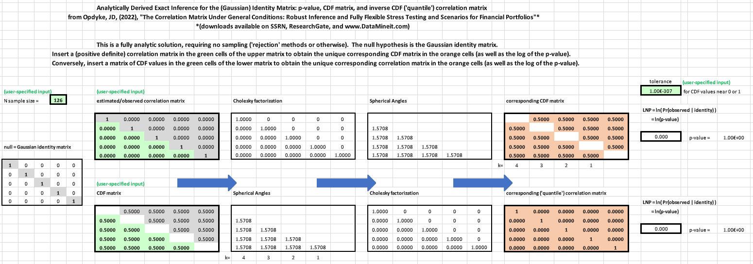
Read the full excel workbook here.
While many papers address one, and sometimes two of the above, none successfully address all three challenges. Herein we follow previous research that utilizes a geometric framework [17,18,19,20] to develop a method that overcomes the obstacles posed by 1.-3. simultaneously, thus providing the finite sample distribution of the correlation matrix under general conditions.
The Non-parametric Angles-based Correlation (NAbC) method A. automatically and efficiently (and analytically in some cases) enforces positive definiteness via reliance on Cholesky factors to remain on the unit hyper-hemisphere; B. allows fully flexible perturbation of ANY COMBINATION of selected cells in the matrix, while holding the rest constant, via a simple, structured reordering of the matrix; C. uses geometric angles distributions to provide more accurate and more robust results when matrices approach singularity and/or extreme values; D. remains reasonably scalable (e.g. matrices 100x100, and larger); and E. remains valid under the most general conditions possible via non-parametric estimation of the angles distributions.
Multivariate distributions based on any copula function, with varying degrees of tail heaviness, serial correlation, non-stationarity, and/or asymmetry pose no problems for NAbC, empirically or computationally.
All results generated by NAbC are consistent with those well established in the Random Matrix Theory literature [21], even while NAbC remains more robust than methods based on spectral distributions. The distribution of the entire correlation matrix is explicitly defined by those of the individual correlation cells, so both are consistently and simultaneously determined. This provides a new ‘distance metric’ that is a p-value for the entire matrix, which has some advantages over traditional, norm-based metrics.
In addition to all the above properties, NAbC remains far more straightforward and easily implemented than other approaches that provide more limited solutions to this problem. Its range of application is as broad as that of the correlation matrix itself. Next steps for further research include extending the methodology to rank-based correlations.

References
[1] Markowitz, H.M., (1952) "Portfolio Selection," The Journal of Finance, 7(1), 77–91.
[2] Black, F. and Litterman, R., (1991), “Asset Allocation Combining Investor Views with Market Equilibrium,” Journal of Fixed Income, 1(2), 7-18.
[3] Meucci, A., “Fully Flexible Views: Theory and Practice,” Risk, Vol. 21, No. 10, pp. 97-102, October 2008
[4] BIS, Basel Committee on Banking Supervision, Working Paper 19, (1/31/11), “Messages from the acamemic literature on risk measurement for the trading book.”
[5] Pearson, K., (1895), “VII. Note on regression and inheritance in the case of two parents,” Proceedings of the Royal Society of London, 58: 240–242.
[6] van den Heuvel, E., and Zhan, Z., (2022), “Myths About Linear and Monotonic Associations: Pearson’s r, Spearman’s ρ, and Kendall’s τ,” The American Statistician, 76:1, 44-52,
[7] Chmielowski, P., (2014), “General covariance, the spectrum of Riemannium and a stress test calculation formula,” Journal of Risk, 16(6), 1–17.
[8] Parlatore, C., and Philippon, T., (2022), “Designing Stress Scenarios,” NBER Working Paper 29901.
[9] Opdyke, JD, (2022) “The Correlation Matrix Under General Conditions: Robust Inference and Fully Flexible Stress Testing and Scenarios for Financial Portfolios,” QuantMindsEdge: Alpha & Quant Investing, June 6, 2022.
[10] Ng, F., Li, W., and Yu, P., (2014), “A Black-Litterman Approach to Correlation Stress Testing,” Quantitative Finance, 14:9, 1643-1649.
[11] Yu, P., Li, W., Ng, F., (2014), “Formulating Hypothetical Scenarios in Correlation Stress Testing via a Bayesian Framework,” The North American Journal of Economics and Finance, Vol 27, 17-33.
[12] Hansen, P., and Archakov, I., (2021), “A New Parametrization of Correlation Matrices,” Econometrica, 89(4), 1699-1715.
[13] Lan, S., Holbrook, A., Elias, G., Fortin, N., Ombao, H., and Shahbaba, B. (2020), “Flexible Bayesian Dynamic Modeling of Correlation and Covariance Matrices,” Bayesian Analysis, 15(4), 1199–1228.
[14] Ghosh, R., Mallick, B., and Pourahmadi, M., (2021) “Bayesian Estimation of Correlation Matrices of Longitudinal Data,” Bayesian Analysis, 16, Number 3, pp. 1039–1058.
[15] Papenbrock, J., Schwendner, P., Jaeger, M., and Krugel, S., (2021), “Matrix Evolutions: Synthetic Correlations and Explainable Machine Learning for Constructing Robust Investment Portfolios,” Journal of Financial Data Science, 51-69.
[16] Taraldsen, G. (2021), “The Confidence Density for Correlation,” The Indian Journal of Statistics, 2021.
[17] Pinheiro, J. and Bates, D. (1996), “Unconstrained parametrizations for variance-covariance matrices,” Statistics and Computing, Vol. 6, 289–296.
[18] Rebonato, R., and Jackel, P., (2000), “The Most General Methodology for Creating a Valid Correlation Matrix for Risk Management and Option Pricing Purposes,” Journal of Risk, 2(2)17-27.
[19] Pourahmadi, M., Wang, X., (2015), “Distribution of random correlation matrices: Hyperspherical parameterization of the Cholesky factor,” Statistics and Probability Letters, 106, (C), 5-12.
[20] Rapisarda, F., Brigo, D., & Mercurio, F., (2007), “Parameterizing Correlations: A Geometric Interpretation,” IMA Journal of Management Mathematics, 18(1), 55-73.
[21] Marchenko, A., Pastur, L., (1967). "Distribution of eigenvalues for some sets of random matrices,” Matematicheskii Sbornik, N.S. 72 (114:4): 507–536.