The right way to be wrong: learning interest rate interpolation

In the previous blog post, we discussed “QLBS: Q-Learner in the Black-Scholes(-Merton) Worlds” by Igor Halperin. In this one, Halperin learns from the asset paths the option pricing and hedging functions simultaneously.

Without necessarily following the exact procedures of the paper “QLBS: Q-Learner in the Black-Scholes(-Merton) Worlds” by Igor Halperin, let’s calculate the final P&L of a hedged option portfolio.

Assuming that: (i) the option is a vanilla call with strike K and time to maturity T (ii) we bought this option and (iii) that interest rates and dividends are equal to zero, we define:

1. Price of the option at the start (t=0): c_K,0 = f₀(S₀, K, T - 0, σ_{K, T, 0}) where σ is some parameter (the reader will have guesses that this parameter should be some kind of volatility) and f is the pricing function that we want to learn
2. Payoff of the option at the maturity (t=T): c_{K, T} = max(S_T - K, 0)
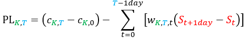
3. The P&L of the option position at the maturity (t=T): c_K, T - c_K,0; we do not expect this to be zero; in fact, this will be anything but zero
4. The amount of the asset chosen to hedge the option position at time t (from 0 to T - 1 day): w_{K, T, t} = f'_t(S_t, K, T - t, σ_{K, T, t}), where f’ is the hedging function associated with the pricing function f.
5. The hedged position at time t is defined as c_{K, t} - w_{K, T, t} S_t + cash_t; we will assume that we are always short the asset and calculate the absolute value of w
6. The cash received when selling the initial hedge position: w_K,T,0 S₀ = f'₀(S₀, K, T - 0, σ_{K, T, 0})S₀
7. The cashflow from the rebalancing of the hedge position at time t: (w_{K, T, t} - w_{K, T, t-1})S_t
8. The cash paid to close the last hedge position (from time T - 1 day) at time T: -w_{K, T, T-1}S_t

After all that, the final P&L of the hedged portfolio can be written as:

or also

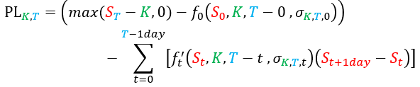
where 

So even if we express f as some approximation or interpolation we can calculate its derivative f’, or vice-versa: if we express f’ as some approximation or interpolation, we can calculate its integral f.

Now there are two ways to look for an optimal function f / f’: You create some metric the looks at the value of the hedged portfolio during the life of the option (for that watch Alexandre Antonov present on “Quantifying Model Performance”) or you create some metric to look at the sum (with some choice of weights) of the final P&Ls of options with different Ks and Ts. Then with either choice you look for the optimal form of the function f / f’ with a choice on how to define the parametrisation of σ_{K, T, t}; if you fix f as the standard Black & Scholes formula and try to find σ_{K, T, t} you are following Dupire’s concept of the breakeven smile / volatility surface.

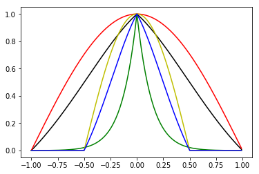
But who said that we need to fix f as the Black & Scholes formula? Why not try to make σ_{K, T, t} as close as possible to a value σ_{T, t} and find the best performing f, and then look at the behavior of σ_{T, t}? We know what f and f’ should look like: f is some curve that sits above the intrinsic value of the option, and therefore f’ starts at 0 and ends at 1 (looking like a sigmoid). And σ_{K, T, t} controls the slope of f’; a volatility smile enables fine control at each point of f’, but which kind of information (or insight) the smile gives us? Is there any predictive power in fixing f and using σ_{K, T, t} to fit everything?

This will be discussed at length in the Option Pricing and Volatility stream at QuantMinds International; but now we will discuss how a similar approach can be used to learn an optimal interest rate interpolation.

Assuming that: (i) we buy a zero-coupon bond with time to maturity T (ii) there are N traded zero-coupon bonds with prices p_{j, t} maturing at times T_j and (iii) that there is an overnight funding rate r_t, we define:

1. Price of the bond at the start (t=0): p_{T, 0} = f₀({p_{j, 0}, T_j}, T - 0, M₀) where M is a matrix of parameters (the reader will have guesses that this matrix should be some kind of covariance matrix) and f is the pricing function that we want to learn
2. Payoff of the bond at its maturity (t=T): p_{T, T} = 1
3. The P&L of the bond position at its maturity (t= T): 1- p_{T, 0} Π^{T-1 day}_t=0 (1+ r_t)^{1 day} ; we do not expect this to be zero; in fact, this will be anything but zero
4. The amount of each traded bond chosen to hedge our bond position at time t (from 0 to T - 1 day): w_{j, T, t} = f'_{j, t}({p_j, t, T_j}, T - t, M_t), where f’ is the hedging function associated with the pricing function f.
5. The hedged position at time t is defined as p_{T, t} - Σ^N_j=1(w_{j, T, t} p_{j, t}) + cash_t ; we will assume that we are by default short the traded bonds and calculate (in most cases) positive values for w
6. The cash received when selling the initial hedge position: Σ^N_j=1(w_{j,t, 0}p_{j, 0}) = Σ^N_j=1 [f'_{j, 0} ({p_{j, 0}, T_j}, t = 0, M₀) p_j,0]
7. The cashflow from the rebalancing of the hedge position at time t: Σ^N_j=1 [w_{j, T, t} - w_{j, T, t-1 day}) p_j, t]
8. The cash paid to close the last hedge position (from time T - 1 day) at time T: - Σ^N_j=1(w_{j, T, T-1 day} p_{j, T-1 day})

After all that, and remembering that we now have the overnight funding rate r_t to apply to every cash balance from one day to another, the final P&L of the hedged portfolio can be written as:

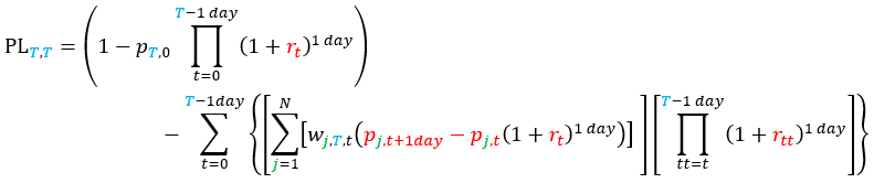
or also:

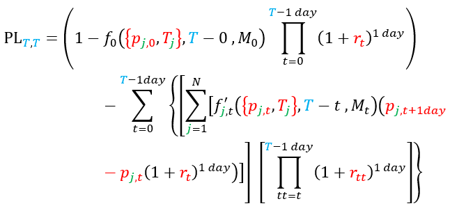
where 

So even if we express f as some approximation or interpolation we can calculate its derivative f’, or vice-versa: if we express f’ as some approximation or interpolation, we can calculate its integral f.

The problem that we have to solve is similar to the option problem, but more things have appeared; instead of just a “volatility”, we have a “covariance” matrix; and now the joint dynamics of the overnight funding rates r_t and the traded bond prices p_{j, t} will make a difference in the final P&L.

So, instead of interpolating just the rates (or yields) of the traded bonds considering the transformation {p_{j, 0}, T_j} → {y_{j, 0}, T_j} and ignoring the joint dynamics of bonds and funding rates, we can try to find the best interpolation for a particular regime of volatility / Central Bank behavior.

And what is the cheat code here?

For the options case we use the smoothness of the “delta” and the peak of the time value around the spot (or forward, in more general terms) to posit a sigmoid structure for f’ and use different strikes, and the monotonicity of total variance to imply a smoother delta for longer maturities.

For bonds we can use a continuity hypothesis and a locality hypothesis (we can drop the locality later), so that weights for each traded bond are equal to 1 at the respective maturity date, 0 before and at the previous traded bond’s maturity, 0 at and after the next traded bond’s maturity date and some smooth function of time to maturity on each side of the bond:

In the presentation, we’ll solve the case where each traded bond has a separate function on the left and on the right and these functions depend on a single parameter; for each time t between 0 and the maturity T of each bond there will be a list of parameters {α_{T, LEFT, j, t}, α_{T, RIGHT, j, t}} that will be found by minimising the sum of the PL_{T, T} as defined above for all possible maturities T in the region where we want to learn our interpolation.

But of course there are ways to improve this method; we can use the initial results to establish some continuity between  {α_{T, LEFT, j, t}, α_{T, RIGHT, j, t}} and  {α_{T, LEFT, j, t+1}, α_{T, RIGHT, j, t+1}} so the learning is more robust and less dependent on particular outliers or lack of volatility. We can use deep networks for interpolation. And we expect that each attendant will figure out how to use this general concept for her particular application.

In short, our initial prices for bonds (and therefore the interpolated rates) at the beginning might seem wrong from the traditional point of view of spline / smoothness rate interpolation, but the traditional approaches say little about the relative importance of the hedge results on the overall performance of bond pricing.

More on this problem and the challenges of learning from market data (regime changes and the need for realised covariance to learn meaningful information) at the QuantMinds International conference in May.