The value of bond convexity
 Convexity means many different things to various people, but how does it relate to duration, bond price and yield? Professor Jessica James, Managing Director and Senior Quantitative Researcher at Commerzbank AG gives us a sneak peak of her presentation ahead of QuantMinds International.
What is convexity? It is a complex subject and there are many different ways of looking at it. Depending upon our point of view, we can say:
- Convexity is a term in an equation connecting bond price and yield
- Convexity is a measure of non-linearity
- Convexity is a function of implied option volatility
- Convexity is great for bond holders
- Convexity is the reason that long dated bonds are bought and sold
Well, looking at the list above, convexity must be something special to do all these things!
Definition of Duration and Convexity
Let’s start from the simplest mathematical definition, and find out how it all works.
The price P of a bond of n years’ tenor, yield y and coupon c is given by (1)
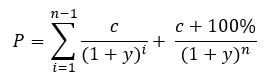
If the yield of the bond changes, of course it is possible to recalculate the new price using the above expression. However, it’s not very intuitive to see how price and yield relate to each other from this. Thus it is usually expressed as (2)
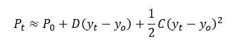
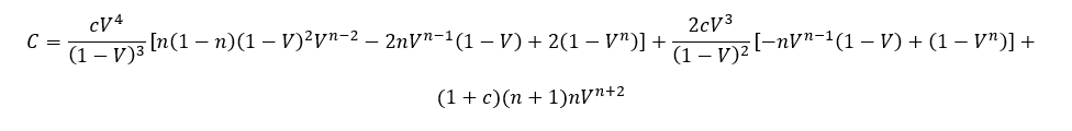
where Pt is the price of the bond at time t, D is the duration, and C is the convexity. D and C are of course the first and second derivatives of price with respect to yield. Can we write these down? Yes, but they are rather long. If you would like to see them, they are in the Appendix (please scroll down). Thus, if an investor holds a bond, with known duration D and convexity C, they can predict the new price it will have at a future time when the yield[1] has changed from y0 to yt.
Relationship of bond price to duration and convexity
How do we use duration? Take a look at the graph below
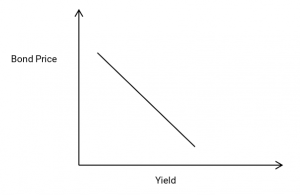
If we can assume that the bond price and the bond yield have a linear relationship, then the duration is the ratio between them, or the slope of the line on the graph. Strictly, there needs to be a minus sign in the definition (2) as well as the slope of the line is negative, though it is usually quoted as a positive number.
If only life were this simple. But the price of the bond is not actually linear with respect to yield; it is more like the below graph.
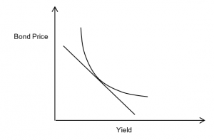
In fact the relationship of price to yield is only modelled well by a linear approximation over a short range; for anything else the curvature of the price-yield relationship is critical, and it is this curvature which is represented by convexity. We can see that this curvature is very beneficial to the owner of the bond. Why? Because the price is always better than the linear approximation would indicate. Thus, the convexity measures the change in duration (or slope of the graph) with respect to yield, or we can say it is the second derivative of bond price with respect to yield. Or, we can simply say that it is a great thing for the bond holder!
Implied convexity value
Though it’s very common to hear that ultra-long bonds are popular due to high convexity, it’s rare to see numbers attached to this convexity value! In part this is because it is a calculation involving a number of assumptions about future yield and volatility levels, so it can only ever be an estimate. Also, the calculation itself is somewhat complex; apart from the rather long closed form solution which we give in the Appendix, it can be done using finite differences, or by multiplying the PV of each cashflow by a factor connected with yield and tenor. Thus it tends to be discussed more qualitatively than quantitatively, which is a pity, as precise comparisons can be useful.
Convexity C, as defined above, is just a coefficient, not a value. What is the value of this nonlinearity? The value of the third term in equation (2) depends on the change in yield, and so the expected value of the convexity of a bond, over the next year for example, will depend upon the expected range of changes of yield over that time.
Now suddenly, we have changed from our fairly deterministic expressions above to something more related to averages, forecasts, and statistics. Because we don’t exactly know the future value of the bond yield, we can’t definitively state what the value of the convexity term will be. However, statistics come to our aid, and if we know the future standard deviation sy of the yield, we can say
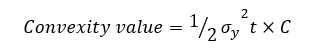
This makes a number of assumptions, none of which are unassailable. It assumes that the future distribution of the yield is known, stationary and lognormal, all of which may be challenged. Nevertheless, it certainly serves to give a useful estimate, and additionally, we do have a ready-made market estimate for sy in the form of the swaption volatility for the relevant tenor and time forward.
We need also to consider what value to use for the coupon of the bond. We can do two things here – the first is to use the yield as the coupon, assuming that the curve will retain its current form over the next year, and the second is to use a forecast value. To obtain forecast values through history, we have created a series of 1y ahead forecasts from the Bloomberg consensus forecast series, which updates each quarter. This is only available for the 10y case but nevertheless is useful.
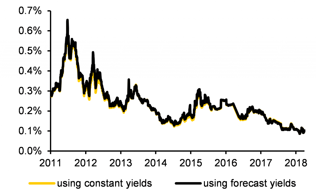
Using all these assumptions, we can go back through history and extract yields and swaption volatilities, to create the graph below of the implied convexity value. Of course, we could also use different volatilities if we felt we could do better than the swaptions, but that starts to become fairly speculative.
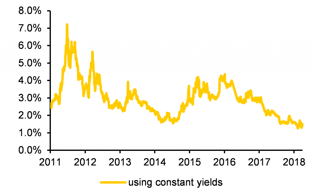
| Implied convexity value, 10y German bonds [2] | Implied convexity value, 50y EUR swaps |
| In % of notional value | In % of notional value |
 |  |
| Source: Bloomberg, Commerzbank AG* Research | Source: Bloomberg, Commerzbank AG* Research |
Two things are worth noting here. The first is the difference in scale; the 50y instruments indeed have a far greater convexity value than the 10y case. The second is that there is almost no difference in using forecast yields vs assuming constant yields. The reason is that the main driver of implied convexity value is the implied swaption volatility, whose range of variation is vastly larger than the relatively modest adjustment in yields.
This is actually somewhat reassuring. When one realises that the implied convexity relies on so many different assumptions, it could be thought that there is little way to obtain a reliable estimate. But when we realise that a single input, the future yield volatility, dominates, at least we have narrowed the range of uncertainty.
Realised convexity value
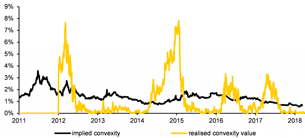
What is also very relevant for bond holders, and also rarely seen, is a measure of how much convexity value a bond turned out to generate! This of course will depend on yield and volatility changes over the period in question, but it is of interest to see how accurate the ‘implied’ convexity is, relative to the actual value realised over time. We compare the implied to the realised convexity value over a 1y period, and show that with some variation, implied and realised values certainly fall into the same range. The main drivers of implied and realised convexity value are implied volatility and change in yield, respectively.
| Implied vs realised convexity for 30y German govt bonds Implied convexity calculated from yield curve, realised from 1y changes, in % notional value |
 |
| Source: Bloomberg, Commerzbank AG* Research |

Appendix
Closed form solutions[i] for Duration (D) and Convexity (C):
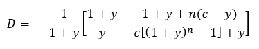
and
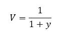
where
*Commerzbank AG is authorised by the German Federal Financial Supervisory Authority and the European Central Bank. Commerzbank AG London Branch is authorised and subject to limited regulation by the Financial Conduct Authority and Prudential Regulation.
[1]A note on the yield term; this is the yield-to-maturity of the bond, which is the equivalent flat interest rate which would duplicate the value of the bond in the current yield curve environment. Thus it changes as the interest rate environment changes and is a useful ‘flat’ rate to use for the bond lifetime.
[2] Note that to obtain a yield curve out to the 50y point, we need to combine bond and swap data.
[i] This definition was first shown to be true in Commerzbank’s Rates Radar: Can you trust forward curves? June 2018, by James, Leister and Rieger, as far as we know. We have not given the proof here, as it is too large to fit in the margin of the paper…