Trading Commodities Using Natural Language Processing

Peter Hafez, Chief Data Scientist at RavenPack is speaking at QuantMinds Americas on Machine Learning and Big Data. Here, he discusses how to separate noise from signal and determine which events have the potential to impact commodity prices.
Being a commodity investor can be a rollercoaster ride, this was clear a few years ago when the prices of energy-related commodities collapsed, led by crude oil. Supply and demand dynamics may dictate the long-term evolution of prices, but, as the recent meltdown of energy commodities has shown, there can be prolonged periods of pricing anomalies. Economic indicators, natural disasters and political upheaval all influence prices, as do commodity-specific issues such as oil spills, gas pipeline leakages and drilling accidents.
Given the vast amount of unstructured textual content available in today’s market, investors often struggle to separate noise from signal and determine which of these events has the potential to impact commodity prices. However, by utilizing the latest advances in Natural Language Processing (NLP), market participants have the ability to detect high-impact events and identify commodity price triggers in real-time.
Researchers from Duke University have previously shown how sentiment on geopolitical and fundamental news can impact oil prices, both in the short-term and long-term. However, in our latest research report “Machine Learning & Event Detection for Trading Energy Futures”, we took a different approach by demonstrating how to take advantage of commodity specific events to predict next-day returns across an energy commodities basket.
We train ten different machine learning algorithms across close to 100 different commodity specific events detected from news, including anything from drilling events to import tax, supply, or inventory increase or decrease events. Whenever a novel event category is detected at least once for a given commodity on a given day, we assign a one (1) to the relevant column in our features matrix, and zero (0) otherwise.
To minimize the prediction bias, we take an ensemble approach by equally weighting our ten ML algorithms. Overall, we find that such portfolios outperform the individual models in eight cases out of ten.
The cumulative return profile, presented in Figure 1, underlines the impressive performance of the ensemble strategy, delivering out-of-sample total returns of 38.8%, while the long-only benchmark has returned -12.8% in comparison.
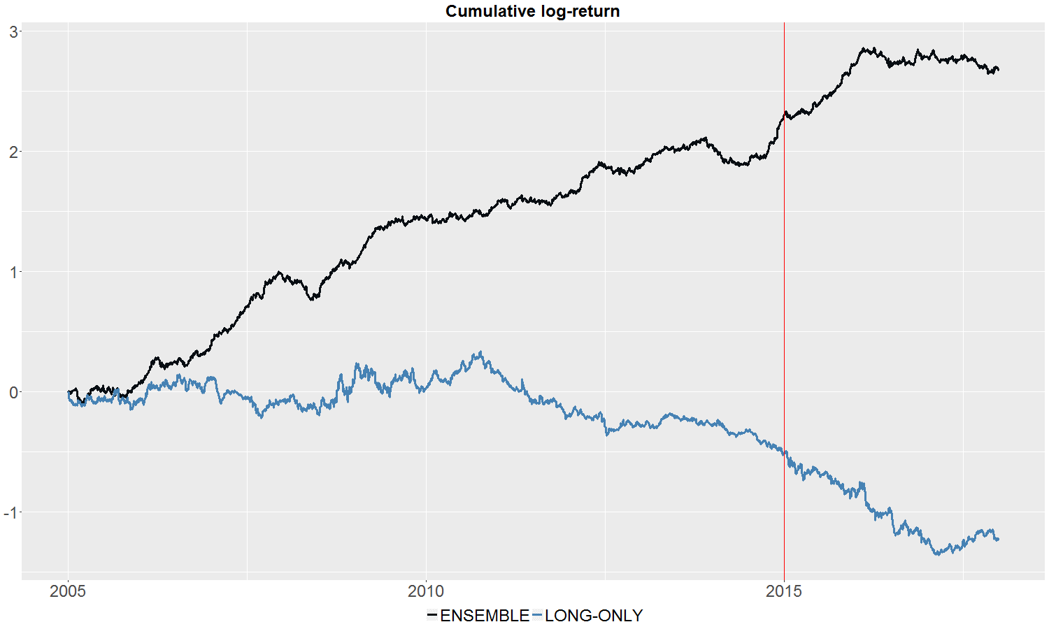
Figure 1: Cumulative log-return
There has been a dearth of volatility in many asset classes of late, including energy commodities. This may help explain the lack of performance towards the end of the out-of-sample period. Our strategy does not take volatility into account when placing a trade, resulting in a lot of small wins and losses lacking a clear direction. We take steps to correct this by acknowledging that higher volatility regimes often provide stronger signals for trading, while we should stay on the sidelines during lower-volatility regimes.
We implement this into practice by imposing a very simple rule: (1) only trade the model whenever short-run volatility (10-days) is above medium-term volatility (21-days), or (2) when the one-day lagged 21-day volatility is above its annual average. When at least one of the conditions is fulfilled we are in a high volatility environment, otherwise we are in a low volatility environment. Table 2 compares the results of the two volatility-conditioned portfolios (high/low) with the ensemble portfolio.
As can be observed, by conditioning on the volatility regime, we are able to find discrepancies in performance. In particular, we find that periods of high volatility yield higher returns, both in absolute and risk-adjusted terms. In particular, the out-of-sample period yields an IR of 1.08 on an annualized return of 16.8% for the high regime compared to 0.92 for our ensemble strategy. Importantly, we improve the per-trade return by nearly 40% in the high strategy from 5.05bps to 6.98bps while the hit ratio improves from 53.9% to 55.0%. These results are further supported by the in-sample evidence – showing that the low volatility signals are yielding significantly worse performance from a statistical significance point-of-view (99%-level).
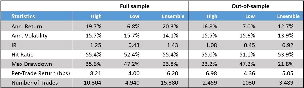
Table 1: Performance statistics for volatility regime-dependent strategies
As an additional filter, we consider whether the one-day lagged returns and predicted returns reveal some regime not captured by the ensemble strategy. Specifically, we create a filter based on the direction of (1) one-day lagged returns and (2) one-day predicted returns. Combining these two rules amount to investigating how well the portfolio does during trending periods (the direction of returns are identical) vs. reversal periods (the direction of returns are distinct). Table 3 compares the results of the trending and reversal portfolios with the ensemble portfolio.
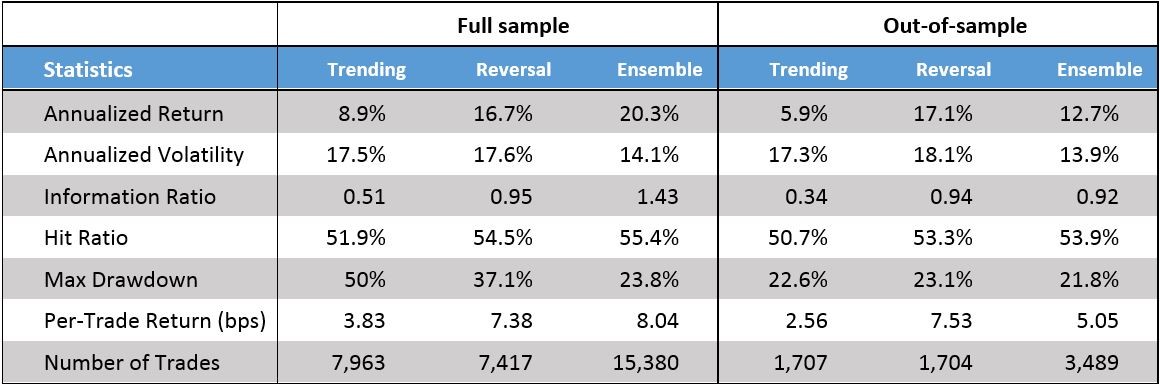
Table 2: Performance statistics for lag-return regime-dependent strategies
Again, we find clear indication that our ensemble strategy can be improved by taking into account certain characteristics of the market and/or model predictions. In particular, by limiting ourselves to trading only during reversal periods – i.e. those periods when the ensemble model’s predicted returns have the opposite sign of the one-day lagged return – we can improve absolute, risk-adjusted and per-trade returns, while lowering costs by staying out of the market at inopportune moments. While the Information Ratio slightly increases from 0.92 to 0.94, absolute return climbs from 12.7% to 17.1% and the per-trade return reaches 7.53bps – an almost 50% improvement on the ensemble strategy. Again, the difference in performance between the trending and reversal strategies is supported by the in-sample evidence showing that the trending strategy is statistically significantly worse than the random benchmark portfolio at a 95% confidence-level.
Figure 2, presents the out-of-sample cumulative return profiles of the ensemble and combine portfolios, where the combine portfolio combines the reversal and high-volatility strategies in equal weight. In terms of performance, the combine strategy delivers an IR of 1.22 out-of-sample driven by an annualized return of 17.0%. This compares with the ensemble strategy’s annualized return of 12.7% and IR of 0.92.
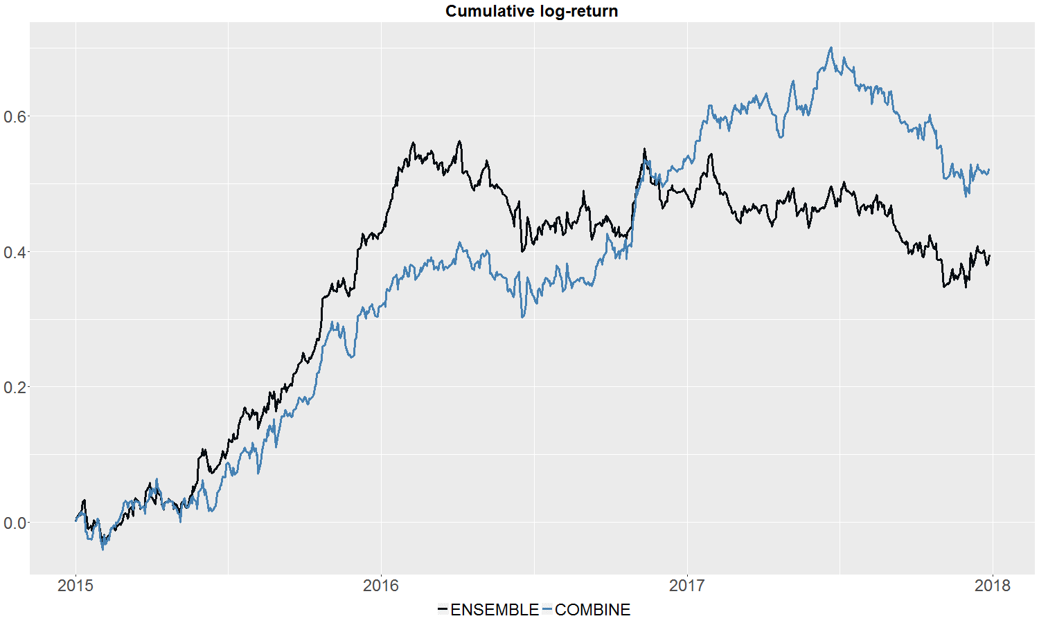
Figure 2: Cumulative out-of-sample log-return for the combine strategy
About RavenPack Data: RavenPack Analytics provides real-time structured sentiment, relevance and novelty data for entities and events detected in unstructured text published by reputable sources. Sources include Dow Jones Newswires, Barron’s, the Wall Street Journal and over 19,000 other traditional and social media sites. RavenPack generates analytics data on over 45,000 listed stocks, top products and services, all major currencies and commodities, financially relevant places and organizations, and key business and political figures. More than 17 years’ worth of historical data is available for backtesting purposes.