Applications of a new Rational Expectations bubble model

Prof. Dr. Jérôme Kreuser, Senior researcher at ETH Zürich Risk Center explores the new expectations bubble model ahead of QuantMinds Americas. Dr. Kreuser will discuss his RE bubble model and its differences from the Log-Periodic-Power-Law-Singularity method and how both methods can exhibit super-exponential growth rates during this year's event.
Yes, you can detect bubbles and leverage returns. We will tell you why you can, how to do it, and when it works.
Much literature suggests that a Rational Expectations bubble model cannot exist. That is often because the bubble component is additive whereas our bubble component is multiplicative relative to a normal price. Details are available from our Efficient Crashes Paper by Kreuser and Sornette that has been submitted for publication to the European Journal of Finance.
Black Swans have become ubiquitous. But most crashes are not Black Swans because they have a probabilistic signature of happening and size. That signature can be exploited to leverage returns. We will show several examples of when, how, and why that works.
What do we mean when we say “bubble”. We assume that the price fluctuates about a “normal price” like Merton’s concept as you might see in the following illustration for Hong Kong.
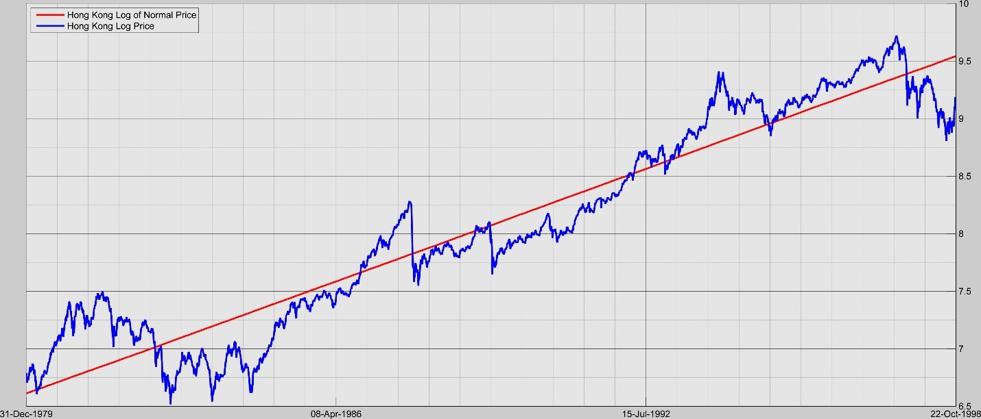
We say that the price has a correction when it moves back toward the normal price. If the correction is fast, we call it a crash when it moves down toward the normal price and a rally when it moves up toward the normal price. If the correction is slow, we call it reverting to the normal price. We may further qualify a crash or rally by its relative mispricing size (ln of normal price minus ln of price).
We then posit a return that fluctuates about the normal price return. It behaves like a discount rate, but we do not impose the requirement that it be a classical discount rate. But rather that it is the rate that defines our Rational Expectation (RE) condition.
We assume our price process is defined as a geometric walk combined with separate crash and rally discrete jump distributions. Such processes are currently being studied widely by Ait-Sahalia, Audrino and Hu, Davis and Lleo, Jacquier and Okou, and others. We combine that price process with our bubble model to postulate our RE condition.
The RE condition implies that the excess risk premium of the risky asset exposed to crashes is an increasing function of the amplitude of the expected crash, which itself grows with the bubble mispricing: hence, the larger the bubble price, the larger its subsequent growth rate (expected return). This positive feedback of price on return is the archetype of super-exponential price dynamics, which has been previously proposed as a general definition of bubbles (Sornette).
We then apply theory that separates geometric random walks from jumps in the historical price data. That allows us to get a crude estimate of ρ, K and σ (with and without jumps).
How to calculate rD and rN ?
We create a simple portfolio of the asset price and a risk-free rate and call this the Optimal Efficient Portfolio, OEP. We calculate the allocation between the asset and the risk-free asset by maximizing the expected log of the value of the OEP (Kelly) assuming our asset follows the RE condition. We estimate rD and rN on several windows of historical data of varied sizes. As we assume that our Kelly method will perform well over time associated with a regime of rather stable stochastics, we select the window sizes and the associated estimates that exhibit optimal performance.
We make all the parameters dynamic in applications. Most importantly the probability becomes dynamic making the process super-exponential. We show how to estimate the accelerating probability as relative mispricing size grows and the price accelerates.
We show one result mitigating the 1929 DJ crash in the following illustration.
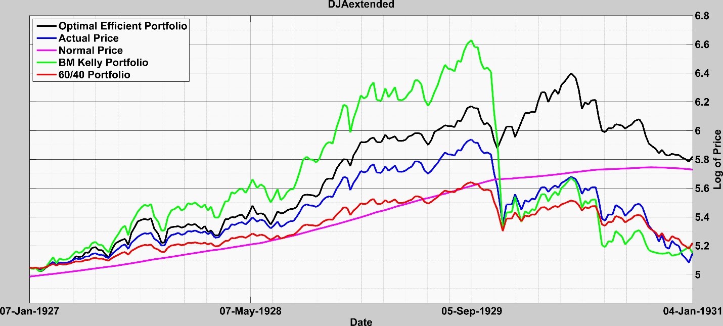
We include the valuation paths for a portfolio using classical Kelly without any estimates of crashes or rallies and a portfolio consisting of 60% of the asset and 40% of the risk-free asset.
We review the details and several examples in our presentation including how, on 19 December 2017, it predicted the Bitcoin crash.