
After three consecutive years of double-digit equity returns investors are faced with a growing list of concerns and unknowns, as market risks and uncertainties continue to grow. Investors are wrestling with the Iran war, uncertain monetary policies, sticky inflation and softening labor market. The uncertainties have resulted in investors focusing on protecting those hard-earned gains.
Asset managers have answered the call by creating strategies to try and protect the 320% cumulative return (S&P 500 index) over the past 10 years but not limit upside potential. These innovative strategies have two things in common - limiting drawdowns and incorporating derivatives. This article takes a deep dive into drawdown risk, why it’s important and how to measure it.
With Americans living longer today, they need to invest in assets with more upside potential and assume a different type of risk – drawdown (loss of capital) risk.
Are you addressing your client’s longevity by including buffered or defined outcome strategies?
Risk has evolved over time as investment environments have changed. Investors originally looked at risk in terms of volatility or standard deviation. In the 1990s, benchmark-relative risks became a main focus. Then the financial crisis arrived, and everything changed. Drawdown risk suddenly became the most pressing issue for managers to contend with.
Investors who had previously asked their advisors whether they were beating a particular benchmark now found themselves asking, “How much money have I lost?”
As markets and risks change, so do investment analytics. Savvy advisors seeking out the best assets for their clients should closely examine fund-manager drawdowns over time.
Take a look at the typical “Growth of $100 Graph” (figure 1). This chart of the S&P 500 index accurately displays overall performance, but it fails to indicate manager drawdowns. Most would focus on the dot com crash of the early 2000s, the Great Financial Crisis or the more-recent pandemic lockdown. It fails to accurately depict other periods of loss years ago. For example, the 1987 market crash doesn’t look too damaging here— but it was.
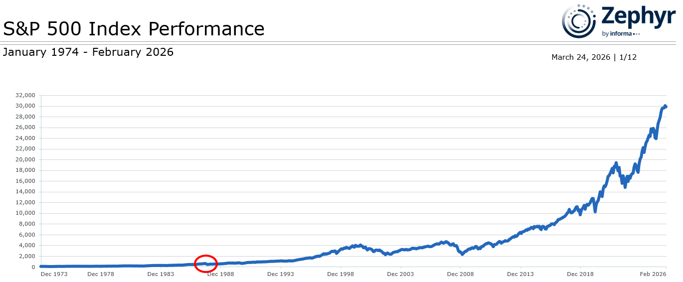 Figure 1: Source - Zephyr
In figure 2, the drawdown graph brings all peak-to-trough losses to scale, and provides a good visual of the depth, duration, and frequency of all losses. It paints a different picture of the 1987 crash; the S&P 500 index lost nearly 30 percent and took almost two years to recover, hardly insignificant.
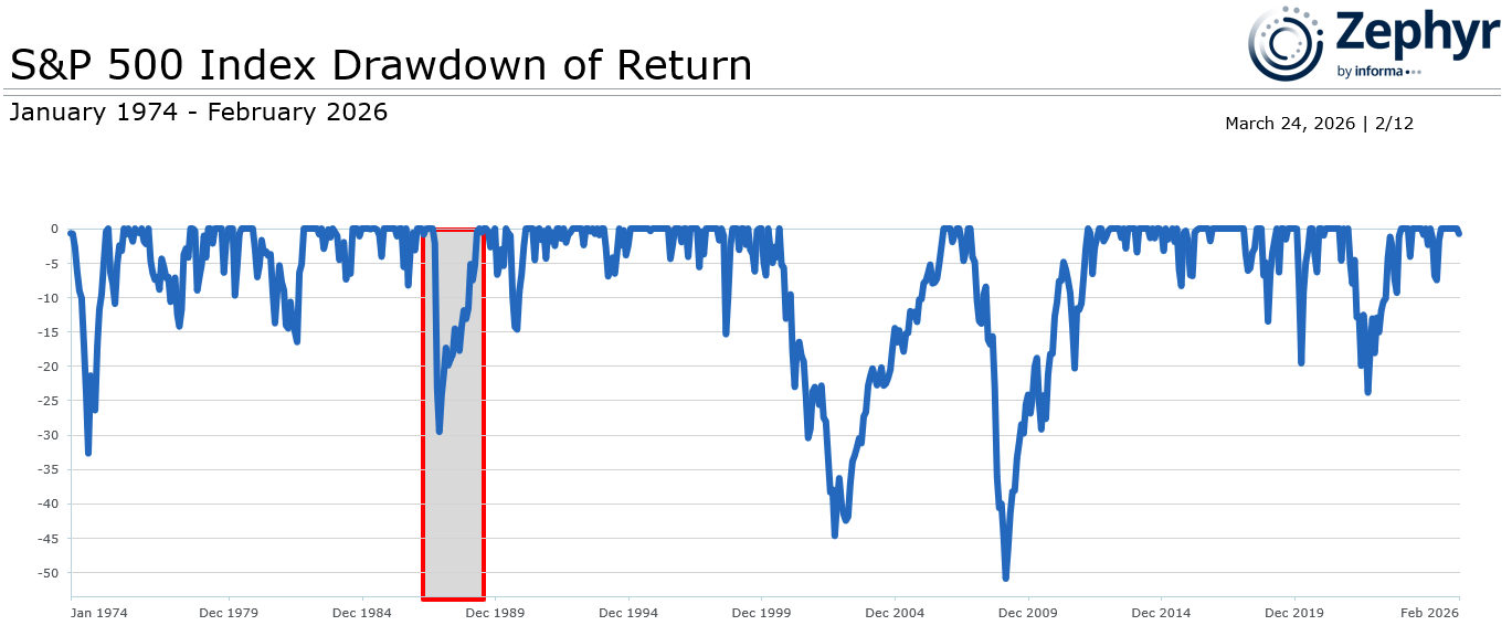 Figure 2: Source - Zephyr
Figure 3 includes a large core mutual fund, which is represented by the blue line. Focusing on the Great Financial Crisis, the S&P 500 index (black line) lost 51 percent from its peak and took over three years to recover after it hit bottom. During that same period, the Large Core Equity fund limited its losses to under 36 percent. By losing less, Large Core Equity was able to preserve more of its capital, providing it with more money to participate in the recovery and regroup in less time than the benchmark (13 months vs. 37 months).
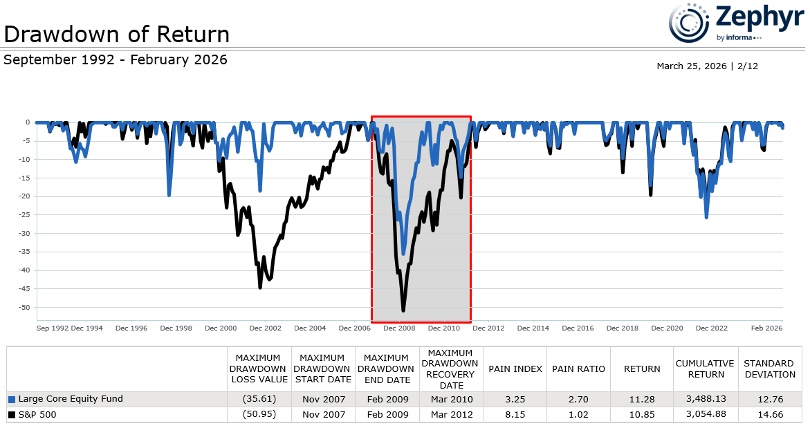 Figure 3: Source - Zephyr
The drawdown table in figure 3 indicates maximum drawdown, or what the largest loss would be if an investor bought at the peak and sold at the trough. In this case it was -35.61 percent. We can also see the timing of this drawdown and the duration (13 Months). The max drawdown is a very telling metric, but it excludes all other drawdowns that occurred over its lifetime. Other metrics are available to address this issue.
Figure 3 also displays the Pain Index and Pain Ratio, statistics which show how a manager performed during a downtrend and quantify their capital preservation tendencies.
The Pain Index measures the depth, duration, and frequency of all periods of losses. (The area within the blue line is the area that the pain index is measuring.) Advisors want to see the periods of loss to be less than that of the benchmark.
An alternative way to measure risk, the index can be used in place of other commonly-used risk statistics like standard deviation and beta. The Pain Index is useful because it only measures drawdown risk, whereas standard deviation considers both upside and downside deviations.
An excellent way to utilize the Pain Index is to compare it to a manager’s excess returns. Figure 4 compares Large Core Equity’s excess return vs. the S&P 500 index (Y-axis) and Pain Index (X-axis) against all the managers that make up the Morningstar Large Blend Universe.
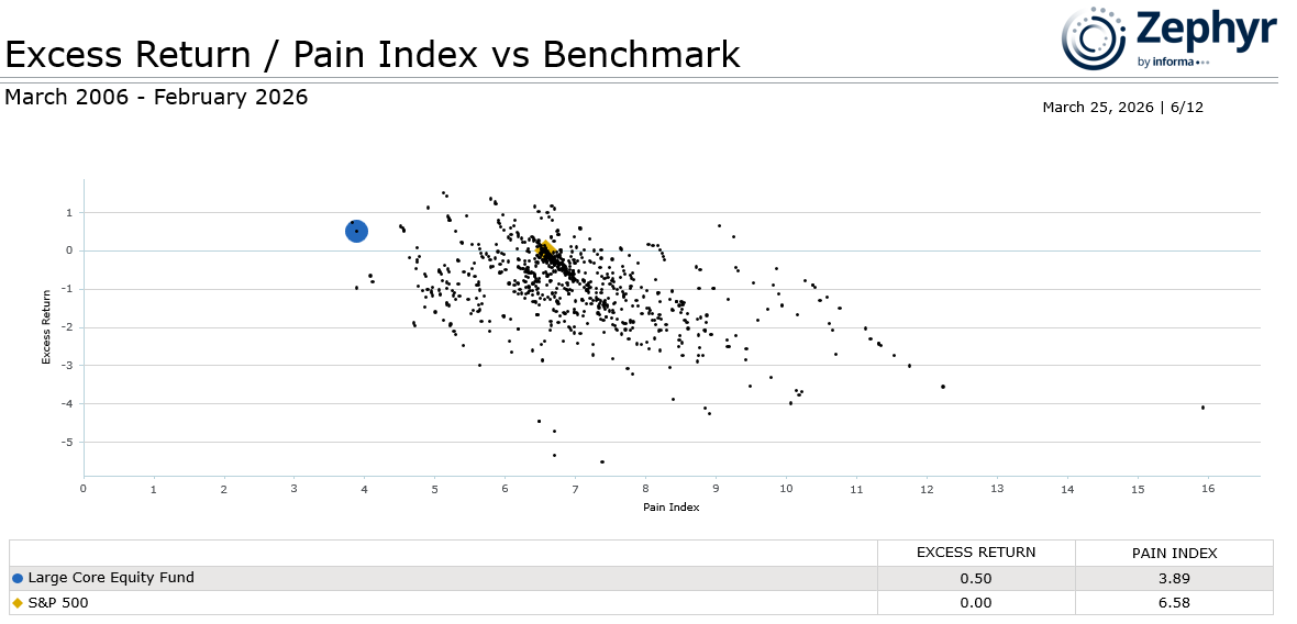 Figure 4: Source - Zephyr
Figure 4 shows how much excess return a manager earns per level of downside risk. Like other return/risk graphs, one looks for managers who plot in the upper left-hand corner, or managers with a lower pain index than that benchmark and positive excess return. Investors concerned about capital preservation want to invest in managers that limit downside losses but also have potential for excess returns.
The Pain Ratio takes the next step and creates a ratio using the manager’s excess return over the risk- free rate, divided by the depth, duration and frequency of losses (Pain Index). If this metric sounds familiar, it should – it’s very similar to the Sharpe Ratio. The difference between the Sharpe Ratio and the Pain Ratio is the risk statistic used as the denominator. The Sharpe Ratio uses standard deviation as its risk measure whereas the Pain Ratio uses the Pain Index. The Pain Ratio shows how much return a manager is earning per level of downside risk. As seen in Figure 3, the Large Core Equity fund has a higher Pain Ratio, so the fund was able to experience more gains over the risk-free rate while experiencing fewer losses.
As markets and risks change, so do investment products and analytics. And by adding drawdown analysis to their research, advisors have even more tools at their disposal to select the best fund managers for their clients.